The question: you have a column of numbers. Where is the middle?
Faced with a new data set, there are five things worth asking, and I would rather you memorised this list than most of the formulas that follow. Professor Leonard opens his course with it and he is right to.
Every descriptive statistic you will learn answers one of those five. If you cannot say which one a number is answering, you do not yet know what it is for. This chapter is question 1; Chapter 3 is questions 2 and 4.
The mean is the balance point:
\[\bar{x} = \frac{\sum_{i=1}^{n} x_i}{n}\]Add everything up, divide by how many. It is the centre of mass: if the values were weights on a ruler, the mean is where you would put your finger to balance it.
The median is the middle value once you have sorted. With an odd number of observations it is the one in the middle; with an even number it is the average of the two straddling the middle.
The mode is the value that occurs most often. That is genuinely all it is — the word means the most. A data set can have one mode, several, or none.
Because they fail differently, and knowing which one to reach for is the actual skill.
The mean is the only one you can do algebra with. $E(aX + b) = aE(X) + b$ works for means and has no counterpart for medians. That is why the entire rest of this course — every standard error, every confidence interval, every test — is built on the mean and not on the median. It is the workhorse, and it is not close.
But the mean feels every observation, including the one somebody typed wrong. That is its weakness, and the next page is the weakness.
The median ignores the sizes of everything except the middle. That makes it blind to outliers — which is a flaw when the outliers are real information, and a virtue when they are not.
The mode is the only one that works on categorical data. You cannot average “economics, biology, history”. You can say which occurs most.
A sample of five values:
\[\{3,\ 7,\ 7,\ 9,\ 14\}\](a) Find the mean, median and mode.
(b) Now suppose the largest value was recorded wrongly — it should have been 44, not 14. Which of the three move, and by how much?
Try (b) in your head before reading on. You should be able to say which two do not move without computing anything.
(a) The mean:
\[\bar{x} = \frac{3 + 7 + 7 + 9 + 14}{5} = \frac{40}{5} = 8\]Sorted, the values are $3,\ 7,\ \mathbf{7},\ 9,\ 14$. With $n = 5$ the middle one is the third, so the median is 7.
The value 7 appears twice and nothing else repeats, so the mode is 7.
(b) With 44 in place of 14:
\[\bar{x} = \frac{3 + 7 + 7 + 9 + 44}{5} = \frac{70}{5} = 14\]The mean has moved by 6. The sorted values are now $3,\ 7,\ \mathbf{7},\ 9,\ 44$ — the middle one is still 7, so the median has not moved at all. Neither has the mode.
One bad value dragged the mean most of the way towards itself. The median never noticed.
That is the entire argument for reporting both, and it is why you see median household income and never mean household income.
The relationship between mean and median tells you the shape.
This is not a rule to memorise so much as a consequence of what the two things are. The mean is pulled by distance, the median only by counting.
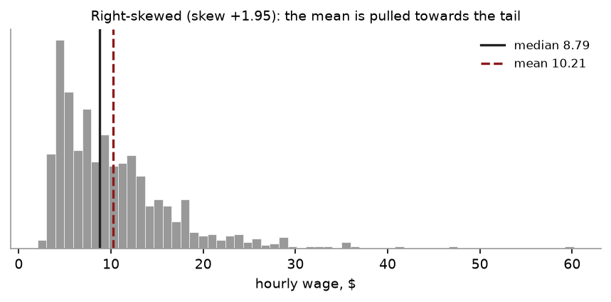
Wages are the standard case, and it is worth seeing on real data rather than taking my word for it. In the CPS extract we use in lab, 1,000 workers:
| Mean hourly wage | $10.21 |
| Median hourly wage | $8.79 |
| Skewness | $+1.95$ |
The mean sits nearly a dollar fifty above the median. A relatively small number of very high earners — the largest in the file is $60.19 — pull the average up while leaving the middle person where she is. If you want to describe what a typical worker earns, $8.79 is the honest number. If you want to describe the total wage bill divided by headcount, $10.21 is. They answer different questions and neither is wrong.
The snippets below assume the header and preamble from Chapter 1 — clear all, the log, and a cd to your own folder.
use "DATA/cps_small.dta", clear
summarize wage
summarize wage, detail
Plain summarize gives you the mean, the standard deviation, and the range.
summarize, detail gives you much more: the percentiles — and the 50th percentile
is the median — plus skewness and kurtosis, and the five largest and smallest
values, which is the fastest outlier check there is.
Stata has no mode in summarize, because the mode is nearly useless for
continuous data: with 1,000 wages measured to the cent, almost every value is
unique. If you need it for a categorical variable, use tabulate and read off the
biggest row.
tabulate educ
import pandas as pd
from scipy import stats

d = pd.read_stata("DATA/cps_small.dta")
w = d["wage"]

print(w.mean())            # 10.2130
print(w.median())          #  8.7900
print(d["educ"].mode())    # 12  -- mode is useful for discrete variables
print(stats.skew(w))       #  1.9533
That is the chapter’s argument as a picture. The long right tail drags the mean (dashed) a dollar and a half above the median (solid), while the median stays with the bulk of the data. Draw it yourself:
import matplotlib.pyplot as plt

plt.hist(w, bins=60, color="#999999", edgecolor="white")
plt.axvline(w.median(), color="#222222", lw=1.6, label=f"median {w.median():.2f}")
plt.axvline(w.mean(), color="#8b1a1a", lw=1.6, ls="--", label=f"mean {w.mean():.2f}")
plt.legend(); plt.show()
Try it on something symmetric. Replace w with d["educ"] and the two lines
almost coincide — which is the point. The gap between mean and median is the skew.
Reporting the mean of a skewed variable without saying so. Not wrong, exactly, but it misleads, and in a report it will be read as “typical”. Give both, or give the median and say why.
Forgetting to sort before taking the median. The median is defined on sorted data. By hand, this is the single most common slip.
Taking the median of an even-sized sample as “one of the two middle values”. It is their average, and the average need not be a value that appears in the data.
Averaging a categorical variable. Stata will do it. The result means nothing.
Assuming the mode is unique. It often is not, and “no mode” is a legitimate answer when nothing repeats.
For ${12,\ 15,\ 15,\ 18,\ 22,\ 24}$ find the mean, median and mode.
A sample of seven houses sold for (in thousands): 180, 195, 210, 215, 230, 245, 1,400. Compute the mean and the median. Which would you report in a newspaper story about house prices, and why?
A data set has mean 50 and median 62. What shape is it, and sketch roughly what the histogram looks like.
Sum is 106, so $\bar{x} = 106/6 = 17.67$. With $n = 6$ the median is the average of the 3rd and 4th: $(15 + 18)/2 = 16.5$. Mode is 15.
Sum is 2,675, so the mean is $382,143. The median is the 4th of seven sorted values: $215,000. Report the median. Six of the seven houses sold for between 180 and 245; the mean describes none of them, and exists only because of one sale that is arguably a different market entirely.
Mean below median means left-skewed — a long tail running to the left. The bulk of the data sits at the high end with a few small values trailing off below.
The ten scores total $9(72) + 92 = 648 + 92 = 740$, so the new mean is 74. The shortcut: the new value is 20 above the old mean, and that surplus is shared over 10 students, so the mean rises by $20/10 = 2$.
Mean: yes, routinely — the mean of ${1, 2}$ is 1.5. Median: yes, whenever $n$ is even and the two middle values differ. Mode: no, never — it is defined as a value that occurs, so it must be one of them.
Ten more. The arithmetic is deliberately light; what is being tested is whether you can say which centre answers the question in front of you.
For the data $12,\ 15,\ 15,\ 18,\ 22,\ 27,\ 31$: (a) Find the mean, median and mode. (b) Is the distribution left- or right-skewed? Say how you can tell from (a).
Add the value 140 to the data in question 1. (a) Recompute the mean and the median. (b) Which moved more, and by how much? (c) What does this tell you about which centre to report for house prices?
Five numbers have a mean of 24. Four of them are $18,\ 22,\ 27,\ 31$. Find the fifth.
A course is graded 20% coursework, 30% midterm, 50% final. A student scores 85, 78 and 92. (a) Find the weighted mean. (b) Find the unweighted mean of the three scores, and explain in one sentence why it is the wrong number to report.
A survey records commuting time in four classes:
| Minutes | 0–10 | 10–20 | 20–30 | 30–40 |
|---|---|---|---|---|
| Households | 8 | 12 | 15 | 5 |
(a) Estimate the mean using class midpoints. (b) Which class contains the median? (c) Why is (a) an estimate rather than the mean?
An investment returns $+10\%$, then $+5\%$, then $-5\%$. (a) Find the arithmetic mean of the three returns. (b) Find the geometric mean return. (c) $100 invested at the start — what is it worth at the end? Which of (a) and (b) reproduces that figure?
A firm reports that its mean salary is $74,000 and its median salary is $46,000. (a) What shape is the salary distribution? (b) The union quotes the median and management quotes the mean. Neither is lying. Explain what each is really saying.
For each, name the centre you would report and why. (a) The most common shoe size a shop should stock. (b) The typical household income of a US county. (c) The average exam mark in a class of 40 with no outliers. (d) The typical brand of car in a car park.
A dataset of 50 values has a mean of 30. Every value is then increased by 4, and the result is doubled. What is the new mean? State the rule you used.
“The mean is the balance point of the data.” Explain what that sentence means arithmetically, using the fact that deviations from the mean sum to zero.
(a) Sum $= 140$, so mean $= 140/7 = 20$. The middle value of seven sorted numbers is the fourth, so median $= 18$. Mode $= 15$, the only repeated value. (b) Right-skewed. Mean $>$ median $>$ mode, which is the signature of a long right tail — the large values 27 and 31 pull the mean up while leaving the middle value where it is.
(a) Sum $= 280$ over 8 values, so mean $= 35$. With eight values the median is the average of the fourth and fifth: $(18+22)/2 = 20$. (b) The mean moved 15 (from 20 to 35); the median moved 2 (from 18 to 20). One observation in eight shifted the mean by three-quarters of its original value. (c) Report the median. House prices have a long right tail and a handful of very expensive sales, and the mean describes none of the houses anyone is actually buying.
The five values sum to $5 \times 24 = 120$. The four given sum to 98. The fifth is $120 - 98 = 22$.
(a) $0.20(85) + 0.30(78) + 0.50(92) = 17 + 23.4 + 46 = 86.4$. (b) The unweighted mean is $255/3 = 85$. It is wrong because it treats the coursework, worth a fifth of the grade, as mattering as much as the final, worth a half — the weights are the question.
(a) Midpoints 5, 15, 25, 35 with frequencies 8, 12, 15, 5. The weighted total is $40 + 180 + 375 + 175 = 770$ over $n = 40$, so the estimated mean is 19.25. (b) With 40 observations the median sits between the 20th and 21st. The cumulative counts are 8, 20, 35, 40 — so the 21st value is in the 20–30 class. (c) Because the individual values were thrown away. Using the midpoint assumes every household in the 20–30 class sits at exactly 25, and unless the values are symmetric within each class that is not true.
(a) $(10 + 5 - 5)/3 = 3.3333\%$. (b) The growth factors are 1.10, 1.05, 0.95, whose product is 1.09725. The geometric mean factor is $1.09725^{1/3} = 1.0314$, so 3.14% a year. (c) $100 becomes $100(1.09725) = $109.73$. Compounding at 3.14% for three years gives $100(1.0314)^3 = $109.73$; compounding at the arithmetic mean of 3.3333% gives $110.34, which is too high. The geometric mean is the one that reproduces the actual outcome, and the arithmetic mean of growth rates always overstates it.
(a) Strongly right-skewed — the mean sits far above the median, so a small number of very large salaries are pulling it up. (b) The median says “half the staff earn under $46,000”, which is a statement about a typical employee. The mean says “total payroll divided by headcount is $74,000”, which is a statement about the wage bill. Both are true; they answer different questions, and the gap between them is itself the interesting number.
(a) Mode — a shop stocks the size most people ask for, and no one wears the mean size. (b) Median — income is right-skewed. (c) Mean — with no outliers it uses every observation and is the most efficient. (d) Mode — brand is nominal, so the mean and median do not exist.
Adding 4 shifts the mean to 34; doubling scales it to 68. The rule is that for a linear transformation, $\overline{aX+b} = a\bar{x} + b$ — here $2(30 + 4) = 68$.
If you place the observations on a number line as equal weights, the mean is the point at which the line balances. Arithmetically, that is the statement $\sum(x_i - \bar{x}) = 0$: the deviations above the mean and the deviations below it sum to exactly the same amount. No other point has that property, which is also why a single extreme value drags the mean so far — it is a long lever arm, and the balance point must move to compensate.