The question: two data sets have the same mean. How else do they differ?
Two factories both average 50 units a day. One produces between 48 and 52; the other swings between 10 and 90. Same mean, and you would run them very differently.
Centre is the first of the five questions from Chapter 2. This chapter is the second and the fourth — variation, and outliers — and it ends with the move that the rest of the course is built on.
The range is maximum minus minimum. It uses two numbers and throws away everything in between, so a single freak value controls it entirely. Report it as a quick sanity check, never as your answer.
The interquartile range is $Q_3 - Q_1$, the width of the middle half. It ignores the extremes by construction, which makes it the spread to pair with a median.
The variance and standard deviation use every observation, and they are what the rest of the course needs.
\[s^2 = \frac{\sum (x_i - \bar{x})^2}{n-1} \qquad\qquad \sigma^2 = \frac{\sum (x_i - \mu)^2}{N}\] \[s = \sqrt{s^2}\]Work from the inside out and it stops looking arbitrary.
$x_i - \bar{x}$ is how far one observation sits from the middle. You cannot simply average these, because $\sum(x_i - \bar{x}) = 0$ always — that is what “balance point” means, and the positives cancel the negatives exactly.
So square them. Squaring kills the signs and, usefully, penalises distant points more than near ones. Add the squares, divide to get an average, and you have the variance.
The variance is in squared units — squared dollars, squared minutes — which nobody has an intuition for. So take the square root, and the standard deviation is back in the units you started with. That is the number to report.
The question that comes up every year.
You are measuring deviations from $\bar{x}$, not from $\mu$. And $\bar{x}$ sits in the dead centre of your particular sample by construction. So your deviations are, on average, slightly too small — they are measured from the most favourable point available rather than from the truth.
Dividing by $n-1$ instead of $n$ inflates them by exactly the right amount to correct for it.
The other way to say the same thing: once you know $\bar{x}$ and any $n-1$ of the values, the last one is forced. Only $n-1$ of the deviations were ever free to vary. That count has a name — degrees of freedom — and it reappears in Chapters 10, 13 and 14 as the parameter of the $t$ distribution. It is the same $n-1$ every time.
For a population you divide by $N$, because there is nothing to correct for. You have everybody.
The five values from Chapter 2: ${3,\ 7,\ 7,\ 9,\ 14}$, with $\bar{x} = 8$.
| $x$ | 3 | 7 | 7 | 9 | 14 |
|---|---|---|---|---|---|
| $x - \bar{x}$ | $-5$ | $-1$ | $-1$ | $1$ | $6$ |
| $(x-\bar{x})^2$ | 25 | 1 | 1 | 1 | 36 |
The deviations sum to zero, as they must — a free check on your arithmetic. The squares sum to 64, so
\[s^2 = \frac{64}{5-1} = 16 \qquad s = \sqrt{16} = 4\]Build that table every time. It is the same table that produces covariance in Chapter 4, and being fast at it is most of the battle on a timed paper.
A standard deviation of 9 is large for shoe sizes and tiny for house prices, so raw standard deviations cannot be compared across variables with different means. The coefficient of variation fixes that:
\[\text{CV} = \frac{s}{\bar{x}}\]A bank’s Branch A has a mean wait of 42 seconds with $s = 6$; Branch B averages 78 seconds with $s = 9$.
\[\text{CV}_A = \frac{6}{42} = 14.29\% \qquad \text{CV}_B = \frac{9}{78} = 11.54\%\]Branch B has the larger standard deviation and is the more consistent of the two relative to its own average. A manager comparing raw standard deviations would get this exactly backwards.
“How many standard deviations from the middle is this?”
Three things about it.
It strips the units. A $z$ of 1.5 means the same thing for dollars, kilograms and test scores, which is what makes comparison across different variables possible at all.
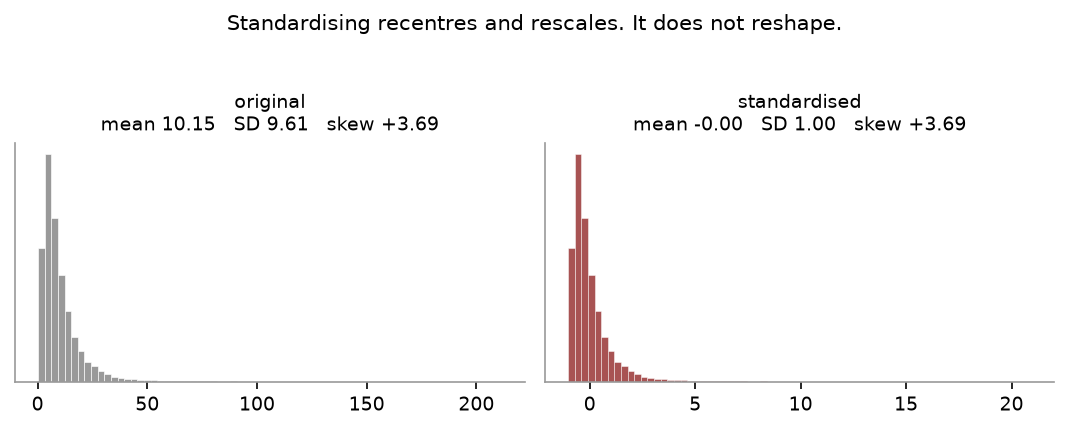
It does not change the shape. Standardise a skewed variable and you get a skewed variable with mean 0 and standard deviation 1. Standardising is not a way of making something normal, and the Stata section below demonstrates it.
And every test statistic in this course is a $z$ in disguise:
\[\frac{\text{what I got} - \text{what I expected}}{\text{how much it typically wobbles}}\]Chapter 14 will put $\bar{x}$ on top and a standard error underneath, but the shape is this one.
For data that is roughly bell-shaped — and only then — the standard deviation has a direct reading:
| within | of the mean |
|---|---|
| $\mu \pm 1\sigma$ | about 68% of observations |
| $\mu \pm 2\sigma$ | about 95% |
| $\mu \pm 3\sigma$ | about 99.7% |
The exact figures are 68.27%, 95.45% and 99.73%. This is where “a $z$ beyond 2 is unusual” comes from, and it is worth memorising because it lets you sanity-check an answer without a table.
The snippets below assume the header and preamble from Chapter 1 — clear all, the log, and a cd to your own folder.
use "DATA/cps_small.dta", clear
summarize wage
summarize wage, detail
summarize gives the standard deviation. summarize, detail adds the percentiles —
$Q_1$ is the 25th, $Q_3$ the 75th, so the IQR is the difference — plus skewness and the
five largest and smallest values, which is the fastest outlier check available.
To standardise a variable:
egen double zwage = std(wage)
summarize zwage
histogram zwage, normal
egen std() subtracts the mean and divides by the standard deviation. summarize will
confirm the new mean is 0 and the new standard deviation is 1 — and the histogram will
show you that the shape has not changed at all. Wage was right-skewed before
standardising and is right-skewed after.
The one thing to watch is ddof. NumPy divides by $n$ by default, which is the
population formula. For a sample you must ask for $n-1$:
import numpy as np

D = [3, 7, 7, 9, 14]

np.std(D)            # 3.5777  -- divides by n.  NOT what you want for a sample
np.std(D, ddof=1)    # 4.0000  -- divides by n-1.  This one.
np.var(D, ddof=1)    # 16.0000
pandas gets this right by default: d["wage"].std() already uses $n-1$. NumPy does
not. It is the single most common silent error when people move between the two.
# coefficient of variation, from the branch example
for name, mean, sd in [("A", 42, 6), ("B", 78, 9)]:
    print(f"{name}: CV = {sd/mean:.4f}")      # A 0.1429   B 0.1154
Both panels are the same 20,000 values. Standardising moved the mean to 0 and set the standard deviation to 1 — and left the skewness identical to four decimal places.
z = (x - x.mean()) / x.std(ddof=1)

print(stats.skew(x), stats.skew(z))    # the same number, twice
If standardising made things normal, the right panel would be a bell. It is not, and this is the cheapest way to settle an argument about it.
Dividing by $n$ when you have a sample. Use $n-1$ unless the data really is the whole population.
Forgetting to square-root. The variance is not the standard deviation, and an answer in squared minutes is almost always a missing square root.
Comparing standard deviations across different variables. Use the coefficient of variation, as the branch example shows.
Applying the empirical rule to skewed data. The 68–95–99.7 figures assume a bell. For a skewed variable they can be badly wrong.
Thinking standardising normalises. It centres and rescales. It does not reshape.
For ${4,\ 8,\ 9,\ 11,\ 13,\ 15}$ compute the range, the mean, the sample variance and the sample standard deviation.
A data set has $\bar{x} = 60$ and $s = 5$. Convert each to a $z$-score: 52, 60, 73.
Two investments: Fund A returns a mean of 8% with $s = 3$; Fund B returns a mean of 22% with $s = 7$. Which is riskier? Defend your answer with a number.
A sample of deviations from the mean is reported as $-3, -1, 0, 2, 3$. Something is wrong. What, and how do you know without any other information?
Scores are bell-shaped with $\mu = 500$, $\sigma = 100$. (a) Roughly what proportion lie between 400 and 600? (b) Between 300 and 700? (c) A score of 780 — is it unusual? Answer with a $z$-score and one sentence.
Range $= 15 - 4 = 11$. Sum is 60, so $\bar{x} = 10$. Deviations $-6, -2, -1, 1, 3, 5$ square to $36, 4, 1, 1, 9, 25$, summing to 76. So $s^2 = 76/5 = 15.2$ and $s = 3.8987$.
$z = (52-60)/5 = -1.60$; $z = (60-60)/5 = 0$; $z = (73-60)/5 = +2.60$. The last is unusual — beyond two standard deviations.
By standard deviation, B. By coefficient of variation, A is riskier: $3/8 = 37.5\%$ against $7/22 = 31.8\%$. Per unit of return, Fund A’s outcome varies more. Either answer is defensible provided you say which measure you used and why — but the CV is the one that compares like with like.
The deviations sum to $+1$, not 0. Deviations from the mean must sum to exactly zero, so either a value or the mean has been computed wrongly. You need nothing else to know that.
(a) 400 and 600 are $\mu \pm 1\sigma$, so about 68%. (b) $\mu \pm 2\sigma$, so about 95%. (c) $z = (780-500)/100 = 2.80$. Yes — nearly three standard deviations above the mean, which the empirical rule puts in the outer 0.3% or so.
Ten more. Several of these can be done without computing a standard deviation at all, which is the point — knowing what the formula does is worth more than being able to grind it.
For the sample $4,\ 8,\ 10,\ 14,\ 19$: (a) Find the mean and set out the deviation table. (b) Find $s^2$ and $s$. (c) Find the range, and say what the range ignores that $s$ does not.
Treat the same five numbers as a whole population. (a) Find $\sigma^2$ and $\sigma$. (b) Which is larger, $s$ or $\sigma$, and why must that always be so?
Verify your answer to 1(b) using the shortcut $\sum x^2 - (\sum x)^2/n$.
Two funds are compared. Fund A has a mean annual return of 8% with a standard deviation of 12%; Fund B has a mean of 3% with a standard deviation of 6%. (a) Which is riskier in absolute terms? (b) Compute the coefficient of variation for each. (c) Which is riskier per unit of return, and why does that question need the CV rather than $s$?
Exam marks have $\mu = 70$ and $\sigma = 8$, and the distribution is bell-shaped. (a) Between which two marks do about 68% of students fall? (b) About 95%? (c) A student scores 86. How unusual is that?
Now suppose the same marks are not bell-shaped, and you know nothing about the shape. (a) What is the most you can say about the fraction within 2 standard deviations? (b) Within 2.5 standard deviations? (c) Why is this bound so much weaker than the answer to 5(b)?
Every value in a dataset with mean 40 and standard deviation 6 is increased by 10. (a) What happens to the mean? (b) What happens to the standard deviation? Explain using the deviation table. (c) Now every value is instead multiplied by 3. What are the new mean and standard deviation?
A student’s score is 72 on a test with mean 65 and standard deviation 10, and 81 on a test with mean 75 and standard deviation 4. On which did they do better relative to the class? Show the comparison.
A dataset has $s = 0$. What does the data look like? Can $s$ be negative?
Explain, in your own words and without the algebra, why the sample variance divides by $n - 1$ rather than $n$. Your answer must mention the word “mean”.
(a) Sum $= 55$, so $\bar{x} = 11$. Deviations: $-7, -3, -1, 3, 8$; squared: $49, 9, 1, 9, 64$, summing to 132. (The deviations summing to zero is the free check: $-7-3-1+3+8 = 0$.) (b) $s^2 = 132/4 = 33.00$ and $s = 5.7446$. (c) Range $= 19 - 4 = 15$. The range uses only the two extreme values and throws away everything in between, so two datasets with the same range can have wildly different spreads. It is also, for that reason, maximally sensitive to a single outlier.
(a) $\sigma^2 = 132/5 = 26.40$ and $\sigma = 5.1381$. (b) $s$ is larger. Both divide the same sum of squares, 132, but $s$ divides by the smaller number, so the quotient is bigger. That is the whole correction: the deviations were taken from $\bar{x}$, which sits in the middle of this particular sample by construction, so they understate the spread around the true $\mu$, and dividing by $n-1$ inflates the answer to compensate.
$\sum x^2 = 16 + 64 + 100 + 196 + 361 = 737$, and $(\sum x)^2/n = 55^2/5 = 605$. The difference is $737 - 605 = 132$, matching the deviation table exactly. The shortcut is faster but tells you nothing about the shape of the data; the deviation table is slower and shows you which observations are doing the damage.
(a) Fund A, with a standard deviation of 12% against 6%. (b) CV$_A = 12/8 = 1.5000$; CV$_B = 6/3 = 2.0000$. (c) Fund B is riskier per unit of return. The question needs the CV because $s$ has units and B’s returns are on a smaller scale — 6% of variation around a 3% mean is proportionally worse than 12% around 8%. Comparing raw standard deviations across series with different means answers a different question from the one asked.
(a) $70 \pm 8$, so about 62 to 78. (b) $70 \pm 16$, so about 54 to 86. (c) $z = (86-70)/8 = 2.00$, so the score is two standard deviations above the mean — at the top edge of the middle 95%, which puts roughly 2.5% of the class above it.
(a) Chebyshev gives at least $1 - 1/2^2 = 0.7500$, so at least 75%. (b) At least $1 - 1/2.5^2 = 1 - 1/6.25 = 0.8400$, so at least 84%. (c) Because it assumes nothing. The empirical rule’s 95% is a statement about a specific shape; Chebyshev’s 75% has to hold for every distribution including the nastiest one anyone can construct, so it is necessarily loose for well-behaved data. The price of needing no assumptions is a weaker conclusion.
(a) The mean becomes 50. (b) It does not change. Each value rose by 10 and so did the mean, so every deviation $x_i - \bar{x}$ is exactly what it was. Shifting the data moves its location, not its spread. (c) Mean $= 120$, standard deviation $= 18$. Multiplying scales every deviation by 3, and since $s$ is in the original units it scales by 3 too — note that $s^2$ scales by 9.
Test 1: $z = (72-65)/10 = 0.7000$. Test 2: $z = (81-75)/4 = 1.5000$. The second score is 1.5 standard deviations above its class mean against 0.7 for the first, so the 81 was the better performance relative to the class, even though the raw gap above the mean was smaller in absolute terms on the test with the tighter spread.
Every value is identical and equal to the mean, so every deviation is zero. $s$ cannot be negative: it is the square root of a sum of squares divided by a positive number, and that sum is zero at best.
The deviations are measured from the sample mean, and the sample mean is itself computed from the very data whose spread you are measuring. It sits, by construction, in the middle of this particular sample rather than at the population’s true centre — so the squared deviations around it are systematically a little too small. Dividing by $n-1$ instead of $n$ makes the answer slightly larger, by exactly the right amount on average. The other way to say it: once you know $\bar{x}$ and any $n-1$ of the observations, the last one is determined, so only $n-1$ of the deviations are free to vary.