The question: when one variable goes up, what does the other do?
Before any formula, plot the two variables against each other. A scatterplot answers most of what you want to know — direction, strength, whether the relationship is a line at all, and whether one odd point is driving everything — and it answers it in a second.
Every number in this chapter can be produced by a variable that looks nothing like what the number suggests. The plot is the defence against that.
It is the same deviation table as Chapter 3, with one change: instead of squaring each $x$ deviation, you multiply it by the matching $y$ deviation.
Every term asks one question: were $x$ and $y$ on the same side of their own means?
Add them up, and the sign tells you the direction of the relationship. That part is genuinely useful.
The size is not, and this is the thing to understand because it is the reason the next section exists. Covariance carries the units of $x$ multiplied by the units of $y$ — dollar-hours, kilogram-years, things nobody has any feel for. Measure the same heights in centimetres instead of metres and the covariance multiplies by 100, while absolutely nothing about the relationship has changed.
Divide the covariance by both standard deviations and the units cancel. What survives is a pure number, and it is always between $-1$ and $+1$.
Correlation is covariance with the units divided out. That is not a loose analogy; it is exactly what the formula does.
| Sign | direction — same as covariance |
| Magnitude | how tightly the points hug a straight line |
| $r = \pm 1$ | the points lie exactly on a line |
| $r = 0$ | no linear relationship |
A rough reading for the magnitude: above 0.8 is strong, 0.4 to 0.8 moderate, below 0.4 weak. Treat those as conventions, not law.
$r$ measures linear association only. Take $y = x^2$ over values of $x$ running symmetrically either side of zero. The relationship is perfect and deterministic, and $r = 0$. A correlation near zero means “no straight-line relationship”, never “no relationship”.
Correlation is not causation. You know the slogan; the useful version is knowing the three ways it fails. $X$ may cause $Y$; $Y$ may cause $X$; or some third variable may cause both. Ice cream sales and drowning deaths correlate strongly, and the third variable is summer.
Five students. $x$ is hours of practice, $y$ is errors made on a task afterwards.
| Practice hours ($x$) | 2 | 4 | 6 | 8 | 10 |
|---|---|---|---|---|---|
| Errors ($y$) | 9 | 7 | 8 | 4 | 2 |
(a) Compute $s_{xy}$. (b) Compute $r$. (c) Errors are re-reported per 100 tasks, so every $y$ is multiplied by 100. What happens to each?
$\bar{x} = 6$ and $\bar{y} = 6$. Build the deviation table:
| $x - \bar{x}$ | $-4$ | $-2$ | $0$ | $2$ | $4$ |
|---|---|---|---|---|---|
| $y - \bar{y}$ | $3$ | $1$ | $2$ | $-2$ | $-4$ |
| product | $-12$ | $-2$ | $0$ | $-4$ | $-16$ |
(a) The products sum to $-34$, so
\[s_{xy} = \frac{-34}{4} = -8.50\](b) The squared deviations give $\sum(x-\bar{x})^2 = 40$ and $\sum(y-\bar{y})^2 = 34$, so $s_x = \sqrt{10} = 3.1623$ and $s_y = \sqrt{8.5} = 2.9155$.
\[r = \frac{-8.50}{(3.1623)(2.9155)} = \frac{-8.50}{9.2195} = -0.9220\]Strong and negative: more practice goes with fewer errors, and the points sit close to a line.
(c) The covariance becomes $-850$ — a hundred times larger. The correlation is unchanged at $-0.9220$, because the 100 appears in $s_{xy}$ and again in $s_y$ and cancels.
That cancellation is the whole reason we report $r$ and not $s_{xy}$.
Variances only add when the covariance is zero. Two positively correlated things rise and fall together, so their total swings more than either alone — which is the argument for diversification, written as algebra.
Memorise it now. It is doing quiet work behind the standard error in Chapter 11.
The snippets below assume the header and preamble from Chapter 1 — clear all, the log, and a cd to your own folder.
use "DATA/cps_small.dta", clear
scatter wage educ
correlate wage educ exper
correlate wage educ, covariance
scatter first, always. correlate gives the correlation matrix; adding
, covariance gives the covariance matrix instead — and comparing the two outputs on
the same variables makes the units point concrete.
To see rescaling do nothing to $r$:
generate wage_cents = wage*100
correlate wage educ
correlate wage_cents educ
Identical correlations. Then run both with , covariance and watch the covariance
multiply by 100.
import numpy as np, pandas as pd

x = [2, 4, 6, 8, 10]
y = [9, 7, 8, 4, 2]

np.cov(x, y, ddof=1)[0, 1]       # -8.5000   the covariance
np.corrcoef(x, y)[0, 1]          # -0.9220   the correlation

pd.DataFrame({"x": x, "y": y}).corr()      # the whole correlation matrix
Note ddof=1 on the covariance, for the same reason as the last chapter.
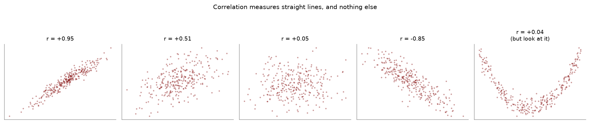
Students can quote “$r$ measures linear association” and still have no picture of what $r = 0.5$ means. Here are five:
The fourth panel is strong and negative. The fifth is the one to remember: a perfect relationship, plainly visible, and $r = +0.04$. Correlation sees straight lines and nothing else.
import matplotlib.pyplot as plt

plt.scatter(x, y, s=12, color="#8b1a1a")
plt.xlabel("practice hours"); plt.ylabel("errors")
plt.show()
Plot before you compute. It takes a second and it is the only thing that reveals curvature, clustering, or a single point driving the whole correlation.
| Stata | Python |
|---|---|
summarize x |
d["x"].describe() |
summarize x, detail |
d["x"].describe() plus stats.skew(d["x"]) |
correlate x y |
np.corrcoef(x, y)[0,1] |
correlate x y, covariance |
np.cov(x, y, ddof=1)[0,1] |
egen z = std(x) |
(x - x.mean()) / x.std(ddof=1) |
scatter y x |
plt.scatter(x, y) |
histogram x, normal |
plt.hist(x, bins=...) |
Reporting covariance as if its size meant something. It depends on your units. Report $r$.
Reading $r = 0$ as “no relationship”. It means no linear relationship.
Skipping the scatterplot. One outlier can create or destroy a correlation, and the plot is the only thing that shows you.
Dividing by $n$ instead of $n-1$ in $s_{xy}$. Same rule as the variance.
Sign errors in the deviation table. Check that both the $x$ and the $y$ deviation rows sum to zero before you multiply. It is free, and it catches most slips.
For the data below compute $\bar{x}$, $\bar{y}$, $s_{xy}$ and $r$.
| $x$ | 1 | 3 | 5 | 7 | 9 |
|---|---|---|---|---|---|
| $y$ | 4 | 7 | 8 | 12 | 14 |
A covariance is computed as 240 for two variables measured in dollars and hours. A colleague says this shows “a very strong relationship”. What is wrong with that claim?
$V(X) = 25$, $V(Y) = 16$, $\text{COV}(X,Y) = -8$. Find $V(X+Y)$ and $V(X-Y)$, and say which is larger and why.
Sketch a scatterplot of ten points with a clear relationship but $r$ close to zero. What kind of relationship did you draw?
In a sample of towns, the number of fire engines sent to a fire correlates strongly and positively with the damage caused. Does sending fewer engines reduce damage? Explain.
$\bar{x} = 5$, $\bar{y} = 9$. Deviations in $x$: $-4, -2, 0, 2, 4$; in $y$: $-5, -2, -1, 3, 5$. Products: $20, 4, 0, 6, 20$, summing to 50, so $s_{xy} = 50/4 = 12.5$. Squared deviations give $\sum(x-\bar{x})^2 = 40$ and $\sum(y-\bar{y})^2 = 64$, so $s_x = 3.1623$, $s_y = 4$, and $r = 12.5/(3.1623 \times 4) = 0.9882$. Very strong and positive.
The size of a covariance has no interpretation on its own, because it carries the product of the two units — here dollar-hours. Restate the hours in minutes and the covariance becomes 14,400 without anything changing. Compute $r$ instead.
$V(X+Y) = 25 + 16 + 2(-8) = 25$. $V(X-Y) = 25 + 16 - 2(-8) = 57$. The difference is more variable, because the two move in opposite directions — so subtracting them compounds the swings while adding them partly cancels.
Any symmetric curved relationship: a parabola, or points on a circle. The relationship is strong but not linear, and $r$ only detects straight lines.
No. Both are driven by a third variable — the size of the fire. Big fires get more engines and cause more damage. This is the “third variable” failure, and sending fewer engines would make the damage worse, not better.
Ten more. Question 5 is the one worth your time — portfolio variance is covariance doing something useful, and it is the reason the topic is in an economics course rather than a maths one.
For the pairs
| $x$ | 2 | 4 | 6 | 8 | 10 |
|---|---|---|---|---|---|
| $y$ | 5 | 9 | 10 | 14 | 17 |
(a) Set out the deviation table and find $s_{xy}$. (b) Find $s_x^2$ and $s_y^2$. (c) Find $r$ and interpret it.
Using the quantities from question 1, find $V(X+Y)$ and $V(X-Y)$. Explain why one is so much larger than the other.
The $x$ values in question 1 are measured in thousands of dollars and the $y$ values in units sold. Suppose $x$ is re-expressed in dollars, so every value is multiplied by 1,000. (a) What happens to $s_{xy}$? (b) What happens to $r$? (c) What does this tell you about which of the two to quote in a report?
A researcher finds $r = -0.85$ between hours of television watched and exam marks, from 200 students. (a) Interpret the number. (b) Give three different explanations for the finding, only one of which is “television lowers marks”.
A portfolio puts 60% of its money in asset 1 ($\sigma_1 = 10$) and 40% in asset 2 ($\sigma_2 = 16$). The correlation between them is 0.30. (a) Find the covariance. (b) Find the variance and standard deviation of the portfolio return. (c) Now suppose the correlation were $-1$ instead. Recompute the standard deviation and say what has happened.
$X$ takes values $-2, -1, 0, 1, 2$ with equal probability, and $Y = X^2$. (a) Find the covariance of $X$ and $Y$. (b) Are $X$ and $Y$ independent? (c) What does this pair of answers tell you about what $r = 0$ does and does not mean?
A report states $s_x = 4$, $s_y = 9$ and $s_{xy} = 40$. One of these three numbers must be wrong. Explain how you know, and state the rule being violated.
For each, say whether you would expect the covariance to be positive, negative, or near zero. (a) Height and weight. (b) Price and quantity demanded. (c) Shoe size and IQ. (d) A firm’s advertising spend and its sales. (e) Hours of sleep and hours spent on a phone at night.
Explain why covariance is almost never reported in a published paper even though correlation is reported constantly, when the two are computed from the same deviation table.
A diversified portfolio of 20 assets has a lower variance than any single asset in it, even though each asset is individually risky. Explain how, using the formula for the variance of a sum.
(a) $\bar{x} = 6$ and $\bar{y} = 11$. Deviations in $x$: $-4, -2, 0, 2, 4$; in $y$: $-6, -2, -1, 3, 6$. Products: $24, 4, 0, 6, 24$, summing to 58. So $s_{xy} = 58/4 = 14.5000$. (b) Squared $x$ deviations sum to 40, so $s_x^2 = 10.0000$. Squared $y$ deviations sum to 86, so $s_y^2 = 21.5000$. (c) $s_x = 3.1623$, $s_y = 4.6368$, so $r = 14.5/(3.1623 \times 4.6368) = 0.9889$. Very strong positive linear association — the points sit almost exactly on a rising straight line.
$V(X+Y) = 10 + 21.5 + 2(14.5) = 60.5000$ and $V(X-Y) = 10 + 21.5 - 2(14.5) = 2.5000$. The two variables move together almost perfectly, so adding them compounds the movement while subtracting them cancels nearly all of it. The difference between the two answers is $4s_{xy} = 58$, and that term is where all the information about co-movement lives.
(a) It is multiplied by 1,000, becoming 14,500. Covariance carries the units of both variables. (b) Nothing. $r$ is unchanged at 0.9889, because the 1,000 appears in both the numerator and in $s_x$ in the denominator, and cancels. (c) Quote $r$. A covariance of 14,500 and a covariance of 14.5 describe the identical relationship, so the number on its own tells a reader nothing until they know the units — whereas $-1 \leq r \leq 1$ always, and 0.99 means the same thing in every field.
(a) A strong negative linear association: students who watch more television tend to have lower marks, and the relationship is tight enough that knowing one tells you a good deal about the other. (b) (i) Television displaces study time, so it causes lower marks. (ii) Reverse causation — students who are struggling and have given up study watch more television. (iii) A third variable, such as household circumstances or a job outside college, drives both. The correlation is identical under all three, and nothing in $r$ distinguishes them.
(a) $\text{COV} = \rho\sigma_1\sigma_2 = 0.30(10)(16) = 48.0000$. (b) $V = 0.6^2(100) + 0.4^2(256) + 2(0.6)(0.4)(48) = 36 + 40.96 + 23.04 = 100.0000$, so the standard deviation is 10.0000 — the same as asset 1 alone, despite 40% of the money sitting in the much riskier asset 2. (c) With $\rho = -1$ the covariance is $-160$, so $V = 36 + 40.96 - 76.8 = 0.1600$ and the standard deviation is 0.4000. The two assets now almost exactly offset each other, and a portfolio of two risky assets is very nearly riskless. This is the whole argument for diversification, and it lives entirely in the covariance term.
(a) $E(X) = 0$ by symmetry, and $E(XY) = E(X^3) = 0$ for the same reason — the cubes $-8, -1, 0, 1, 8$ cancel in pairs. So $\text{COV} = E(XY) - E(X)E(Y) = 0 - 0 = 0$. (b) No. $Y$ is a deterministic function of $X$: tell me $X$ and I know $Y$ exactly. Nothing could be less independent. (c) $r = 0$ rules out a linear relationship and nothing else. Here the relationship is perfect and the correlation cannot see it, because the parabola rises on one side and falls on the other and the two halves cancel in the deviation products. A scatterplot would show it immediately, which is why you plot before you compute.
Dividing out gives $r = 40/(4 \times 9) = 40/36 = 1.1111$, and a correlation cannot exceed 1. The rule is $|s_{xy}| \leq s_x s_y$: the covariance is bounded by the product of the two standard deviations, with equality only when the points lie exactly on a straight line. Here the reported covariance is larger than that product, so at least one of the three figures is mistyped. This is a worthwhile check to run on any table you are handed — it costs one multiplication and catches a transposed digit.
(a) Positive. (b) Negative. (c) Near zero. (d) Positive. (e) Negative.
Because the magnitude of a covariance is uninterpretable without knowing the units of both variables, and changing either unit changes the number without changing the relationship. Correlation is the same quantity with the units divided out, bounded between $-1$ and $1$, so a reader can judge it on sight. The covariance still does all the work — it is what gets reported whenever the units matter, as in the portfolio variance above.
$V(\sum X_i) = \sum V(X_i) + \sum\sum_{i \neq j}\text{COV}(X_i, X_j)$. The variance terms are all positive and cannot be reduced, but the covariance terms can be small, zero, or negative. With 20 assets there are 20 variance terms and 380 covariance terms, so the covariances dominate the sum — and if the assets are weakly or negatively correlated, those 380 terms drag the total far below what the individual variances alone would suggest. Diversification is not about owning many things; it is about owning things whose covariances are low.