The question: how do you put a number on “how likely”?
Chapters 1 to 4 described data you have. Everything from here on describes data you might get — and the bridge is probability.
The connection is the one from Chapter 1: your sample arrived by a random process. To say anything careful about how far $\bar{x}$ might sit from $\mu$, you need a language for randomness. This chapter is that language, and it is only four rules.
An experiment is any process with an uncertain outcome. The sample space is the set of all possible outcomes. An event is a collection of outcomes you care about.
Roll a die: the sample space is ${1,2,3,4,5,6}$, and “even” is the event ${2,4,6}$.
Probabilities obey two rules so basic they are easy to forget: every probability lies between 0 and 1, and the probabilities of all outcomes in the sample space sum to exactly 1. If your answer is 1.4 or $-0.2$, stop.
The cheapest trick available, and the one students under-use.
Whenever a question says “at least one”, try the complement first. “At least one” covers many separate cases; “none” is a single case. Computing one thing and subtracting from 1 beats computing eight things and adding.
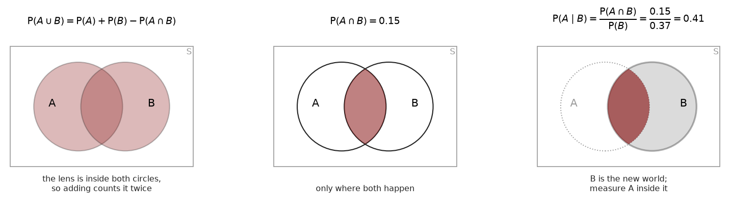
$A \cup B$ is “$A$ or $B$ or both”. You subtract the overlap because adding the two probabilities counts anything in both twice.
When $A$ and $B$ cannot happen together — mutually exclusive — the overlap is empty and the rule simplifies to $\mathrm{P}(A) + \mathrm{P}(B)$. But check that it really is empty rather than assuming.
Read it as: you have been told $B$ happened, so shrink the world down to $B$ and measure $A$ inside it.
That phrase — shrink the world — is the only intuition you need. The denominator is the new world; the numerator is the part of it where $A$ also holds. It is why conditional probabilities are so easy to read off a table, as the worked example shows.
This is Rule 3 rearranged, and it holds always.
It collapses to the familiar $\mathrm{P}(A)\mathrm{P}(B)$ only when $A$ and $B$ are independent — which Chapter 6 takes up properly. Multiplying probabilities without checking independence is the most common error in this material.
These two get confused constantly, and they are close to opposites.
| Mutually exclusive | Independent | |
|---|---|---|
| Means | cannot both happen | knowing one tells you nothing about the other |
| $\mathrm{P}(A \cap B)$ | $0$ | $\mathrm{P}(A)\mathrm{P}(B)$ |
| $\mathrm{P}(A \mid B)$ | $0$ | $\mathrm{P}(A)$ |
If $A$ and $B$ are mutually exclusive and $B$ happens, you know for certain $A$ did not. That is the strongest possible dependence. Mutually exclusive events with non-zero probabilities are never independent.
A credit union classifies 400 loan applications by outcome and by borrower type:
| First-time | Repeat | Total | |
|---|---|---|---|
| Approved | 180 | 120 | 300 |
| Declined | 70 | 30 | 100 |
| Total | 250 | 150 | 400 |
(a) What is the probability an application was approved?
(b) Approved and from a repeat borrower?
(c) Approved or from a repeat borrower?
(d) Approved, given it came from a repeat borrower?
(a) The approved row total over the grand total:
\[\mathrm{P}(A) = \frac{300}{400} = 0.75\](b) The single cell where both hold:
\[\mathrm{P}(A \cap R) = \frac{120}{400} = 0.30\](c) Addition rule, subtracting the overlap:
\[\mathrm{P}(A \cup R) = \frac{300}{400} + \frac{150}{400} - \frac{120}{400} = 0.75 + 0.375 - 0.30 = 0.825\](d) Shrink the world to repeat borrowers — the 150 in that column — and ask how many were approved:
\[\mathrm{P}(A \mid R) = \frac{120}{150} = 0.80\]Notice you can read (d) straight off the table without the formula. That is the whole point of “shrink the world”: the denominator becomes the column total instead of 400.
A bonus observation. $\mathrm{P}(A) = 0.75$ but $\mathrm{P}(A \mid R) = 0.80$. Knowing the applicant is a repeat borrower changes the probability of approval, so these two events are not independent — which is Chapter 6’s test, arriving early.
Contingency tables are where most probability questions on an exam live, so get the pattern fixed:
| You want | Denominator |
|---|---|
| a joint probability, $\mathrm{P}(A \cap B)$ | the grand total |
| a marginal probability, $\mathrm{P}(A)$ | the grand total |
| a conditional probability, $\mathrm{P}(A\mid B)$ | the row or column total for $B$ |
Everything else is reading the right cell.
The snippets below assume the header and preamble from Chapter 1 — clear all, the log, and a cd to your own folder.
Probability is mostly pencil work, but a contingency table is one command:
use "DATA/cps_small.dta", clear
tabulate female black
tabulate female black, cell
tabulate female black, row
Plain tabulate gives the counts. , cell turns every cell into a proportion of the
grand total — those are your joint probabilities. , row makes each row sum to 1 —
those are conditional probabilities given the row variable.
Running all three on the same table is the fastest way to see that joint, marginal and conditional are three different divisions of the same counts.
The left panel is the addition rule and why it has a minus sign: shading both circles covers the lens twice, so you subtract it once to put it right. The middle panel is the intersection alone. The right panel is conditioning, which the next chapter takes up — $B$ becomes the whole world and $A$ is measured inside it.
import pandas as pd

d = pd.read_stata("DATA/cps_small.dta")

pd.crosstab(d.female, d.black)                      # counts
pd.crosstab(d.female, d.black, normalize="all")     # JOINT probabilities
pd.crosstab(d.female, d.black, normalize="index")   # CONDITIONAL, given the row
pd.crosstab(d.female, d.black, margins=True)        # with the totals
Those three normalize options are exactly the three divisions from the chapter.
"all" divides by the grand total; "index" divides by the row total, which is
conditioning on the row. Running all three on one table is the quickest way to see
that joint, marginal and conditional are three ways of dividing the same counts.
| Stata | Python |
|---|---|
tabulate x y |
pd.crosstab(d.x, d.y) |
tabulate x y, cell |
pd.crosstab(d.x, d.y, normalize="all") |
tabulate x y, row |
pd.crosstab(d.x, d.y, normalize="index") |
count if x == 1 |
(d.x == 1).sum() |
Multiplying without independence. $\mathrm{P}(A \cap B) = \mathrm{P}(A)\mathrm{P}(B)$ needs justification every single time.
Forgetting to subtract the overlap in the addition rule.
Confusing $\mathrm{P}(A \mid B)$ with $\mathrm{P}(B \mid A)$. These are different numbers and the difference matters enormously — Chapter 6 is largely about it.
Treating mutually exclusive as independent. They are near-opposites.
Probabilities outside $[0,1]$. Always sanity-check the final number.
$\mathrm{P}(A) = 0.55$, $\mathrm{P}(B) = 0.40$, $\mathrm{P}(A \cap B) = 0.22$. (a) Find $\mathrm{P}(A \cup B)$. (b) Find the probability neither occurs. (c) Find $\mathrm{P}(A \mid B)$. (d) Are $A$ and $B$ independent?
A machine produces items independently, each defective with probability 0.04. Six are drawn. Find the probability that at least one is defective, and say why the complement is the sensible route.
Of 500 commuters, 300 take the bus, 150 cycle, and 40 do both at different times. Find the probability a randomly chosen commuter does neither.
Explain, in your own words and without formulas, why two mutually exclusive events with non-zero probability cannot be independent.
A table shows $\mathrm{P}(A) = 0.6$, $\mathrm{P}(B) = 0.5$ and $\mathrm{P}(A \cap B) = 0.30$. A classmate concludes the events must be mutually exclusive. What has gone wrong, and what are they actually?
(a) $0.55 + 0.40 - 0.22 = 0.73$. (b) $1 - 0.73 = 0.27$. (c) $0.22/0.40 = 0.55$. (d) Yes. $\mathrm{P}(A \mid B) = 0.55 = \mathrm{P}(A)$. Equivalently $0.55 \times 0.40 = 0.22$, which matches the given joint probability.
$\mathrm{P}(\text{none defective}) = 0.96^6 = 0.7828$, so $\mathrm{P}(\text{at least one}) = 1 - 0.7828 = 0.2172$. Directly, “at least one” would need the six separate cases $X = 1$ through $X = 6$ added together. The complement is one calculation instead of six.
$\mathrm{P}(\text{bus or cycle}) = (300 + 150 - 40)/500 = 410/500 = 0.82$, so neither is $1 - 0.82 = 0.18$.
If they are mutually exclusive and you learn that one happened, you immediately know the other did not — its probability drops to zero. Learning something that changes the other’s probability that drastically is the opposite of “tells you nothing”, which is what independence requires.
They have confused the two ideas. $\mathrm{P}(A \cap B) = 0.30$ is not zero, so the events plainly can occur together and are not mutually exclusive. In fact $0.6 \times 0.5 = 0.30$ exactly, so they are independent.
Ten more. Most probability mistakes at this level are not arithmetic — they are reading $\mathrm{P}(A \mid B)$ when the question asked for $\mathrm{P}(B \mid A)$, or multiplying when the draws are not independent. These are built to catch both.
Two hundred graduates are classified by whether they took a statistics course and whether they were employed within six months:
| Employed | Not employed | Total | |
|---|---|---|---|
| Took stats | 60 | 40 | 100 |
| Did not | 50 | 50 | 100 |
| Total | 110 | 90 | 200 |
(a) $\mathrm{P}(\text{employed})$. (b) $\mathrm{P}(\text{took stats and employed})$. (c) $\mathrm{P}(\text{employed} \mid \text{took stats})$. (d) $\mathrm{P}(\text{took stats} \mid \text{employed})$. (e) Are the two events independent? Show the check.
Why are the answers to 1(c) and 1(d) different? State in words what each one is the answer to.
$\mathrm{P}(A) = 0.4$, $\mathrm{P}(B) = 0.5$, $\mathrm{P}(A \cap B) = 0.2$. (a) Find $\mathrm{P}(A \cup B)$. (b) Find $\mathrm{P}(A \mid B)$. (c) Are $A$ and $B$ independent? Mutually exclusive? Answer both.
A machine produces items that are defective 20% of the time, independently. (a) Find the probability all three of the next three are good. (b) Find the probability at least one of the three is defective. (c) Which of these was easier to compute directly, and why does the complement rule exist?
A box holds 10 components, 3 of them faulty. Two are drawn without replacement. (a) Find the probability both are faulty. (b) Find the probability both are faulty if the draws are with replacement. (c) Explain which rule changed between (a) and (b).
In the same box of 10 with 3 faulty, two are drawn without replacement. Find the probability that exactly one is faulty.
A student says: “Mutually exclusive events are independent, because if one happens the other cannot, so they have nothing to do with each other.” Explain why this is exactly backwards, using $\mathrm{P}(A \mid B)$.
Of a firm’s invoices, 70% are domestic and 30% foreign. Of domestic invoices 5% are paid late; of foreign invoices 20% are. (a) Draw the tree and find the probability a randomly chosen invoice is paid late. (b) What fraction of all invoices are foreign and late?
A fair coin is tossed four times. (a) Find the probability of four heads. (b) A gambler who has just seen three heads says the next toss is “due” to be tails. What probability does the gambler have in mind, and what is the correct one?
Explain why $\mathrm{P}(A \cap B) = \mathrm{P}(A)\mathrm{P}(B)$ is a test for independence rather than a rule you may always apply.
(a) $110/200 = 0.5500$. (b) $60/200 = 0.3000$. (c) $60/100 = 0.6000$. (d) $60/110 = 0.5455$. (e) Independence requires $\mathrm{P}(\text{stats} \cap \text{employed}) = \mathrm{P}(\text{stats})\mathrm{P}(\text{employed})$, that is $0.30 = 0.5(0.55) = 0.2750$. It does not, so the events are not independent. Equivalently, $\mathrm{P}(\text{employed} \mid \text{stats}) = 0.60$ against an unconditional 0.55 — knowing someone took the course changes the probability.
(c) takes the 100 students who took statistics as the denominator and asks what fraction of them were employed. (d) takes the 110 employed graduates as the denominator and asks what fraction of them took statistics. Different denominators, so different numbers, even though the numerator — the 60 people in both groups — is the same. Mixing the two up is the single most common error in this chapter and the next.
(a) $0.4 + 0.5 - 0.2 = 0.7000$. (b) $0.2/0.5 = 0.4000$. (c) Independent: $\mathrm{P}(A \mid B) = 0.40 = \mathrm{P}(A)$, so yes — or equivalently $0.4(0.5) = 0.2$ as required. Mutually exclusive: no, since $\mathrm{P}(A \cap B) = 0.2 \neq 0$. Note that two events can be independent and overlapping at once; the two ideas are unrelated.
(a) $0.8^3 = 0.5120$. (b) $1 - 0.8^3 = 0.4880$. (c) (a) was easier, which is the point. “At least one” would otherwise require adding the cases of exactly one, exactly two and exactly three defective; the complement rule replaces three calculations with one, because the opposite of “at least one defective” is the single event “all good”.
(a) $\dfrac{3}{10} \times \dfrac{2}{9} = \dfrac{6}{90} = 0.0667$. (b) $0.3 \times 0.3 = 0.0900$. (c) The multiplication rule. Without replacement the draws are dependent, so the second factor is the conditional probability $\mathrm{P}(B \mid A) = 2/9$ — one faulty component has been removed from a box now holding nine. With replacement the draws are independent and the conditional probability equals the unconditional one.
Two routes give exactly one faulty: faulty then good, or good then faulty. $\dfrac{3}{10}\cdot\dfrac{7}{9} + \dfrac{7}{10}\cdot\dfrac{3}{9} = \dfrac{21}{90} + \dfrac{21}{90} = \dfrac{42}{90} = 0.4667$. Forgetting the second route and reporting 0.2333 is the standard error here.
It is backwards because mutually exclusive events are maximally dependent. If $A$ and $B$ cannot both happen then $\mathrm{P}(A \mid B) = 0$, and unless $\mathrm{P}(A)$ was zero to begin with, that is not equal to $\mathrm{P}(A)$ — learning $B$ occurred has told you everything about $A$, namely that it did not. Independence means learning $B$ tells you nothing; exclusivity means it tells you everything.
(a) $\mathrm{P}(\text{late}) = 0.70(0.05) + 0.30(0.20) = 0.035 + 0.060 = 0.0950$. (b) $0.30(0.20) = 0.0600$ — six per cent of all invoices. Note that foreign invoices are 30% of the book but supply $0.06/0.095 = 63.16\%$ of the late ones, which is the kind of number the finance department actually wants.
(a) $0.5^4 = 0.0625$. (b) The gambler is thinking of $\mathrm{P}(\text{four heads}) = 0.0625$ and concluding a fourth head is unlikely. But that probability applied before any tosses. Three heads have already happened, the coin has no memory, and the probability of tails on the fourth toss is 0.5. The gambler’s fallacy is applying an unconditional probability to a situation where the conditioning information is already in hand.
Because it is a statement that happens to be true for some pairs of events and false for others, and which one you have is an empirical matter. Applying it to dependent events — drawing without replacement, or anything where one outcome shifts the odds of another — gives a confidently wrong answer with no warning sign. The general rule is always $\mathrm{P}(A \cap B) = \mathrm{P}(A)\mathrm{P}(B \mid A)$; the product form is what that reduces to in the special case where $\mathrm{P}(B \mid A)$ happens to equal $\mathrm{P}(B)$.