The question: you run the same trial $n$ times. How many will succeed?
Chapter 7 gave you machinery for any discrete random variable — but it needed a table of probabilities handed to you. This chapter is the first case where you can build the table from a description of the situation.
That is the trade a named distribution offers: accept a few assumptions about how the data arose, and every probability follows from a formula. No table required.
It is only binomial if all four hold. Checking them is worth marks on its own, and it is the honest reason half of real-world “binomial” problems are not.
Condition 3 is the one that quietly fails most often. Drawing without replacement from a small population changes $p$ as you go — take two cards from a deck and the second draw’s probabilities depend on the first. The usual rule of thumb is that sampling without replacement is close enough to binomial when the sample is under about 5% of the population.
Satisfy conditions 2, 3 and 4 with $n = 1$ and you have a Bernoulli trial — a single success-or-failure experiment.
The binomial is just $n$ Bernoullis added together. That is the quickest way to see why $E(X) = np$: it is $n$ copies of $p$. It is also why Chapter 12’s claim that the binomial goes normal is not a separate fact — it is the Central Limit Theorem applied to a sum.
Read it in three pieces, because then you never have to memorise it.
$p^k$ — the probability of $k$ successes, if they all happened first.
$(1-p)^{n-k}$ — the probability that the remaining $n - k$ trials all fail.
$\binom{n}{k}$ — the number of different orders in which those $k$ successes could have occurred. Three successes in ten trials could be the first three, or the last three, or scattered; each arrangement has the same probability, and the coefficient counts them.
And the summary measures:
\[E(X) = np \qquad\qquad V(X) = np(1-p) \qquad\qquad \sigma = \sqrt{np(1-p)}\]Thirty per cent of items coming off a production line need rework. Ten items are drawn independently.
(a) Check the four conditions.
(b) Find $\mathrm{P}(X = 3)$.
(c) Find $\mathrm{P}(X \leq 2)$.
(d) Find $E(X)$ and $\sigma$.
(a) $n = 10$ is fixed; each item either needs rework or does not; $p = 0.30$ is constant; the items are drawn independently. All four hold, so $X \sim \text{Bin}(10, 0.3)$.
(b)
\[\mathrm{P}(X=3) = \binom{10}{3}(0.3)^3(0.7)^7 = 120 \times 0.027 \times 0.0823543 = 0.2668\](c) “At most 2” means $X = 0$, 1 or 2, so three terms added:
\[\mathrm{P}(X \le 2) = \binom{10}{0}(0.7)^{10} + \binom{10}{1}(0.3)(0.7)^{9} + \binom{10}{2}(0.3)^2(0.7)^{8} = 0.3828\](d)
\[E(X) = 10(0.3) = 3.0 \qquad \sigma = \sqrt{10(0.3)(0.7)} = \sqrt{2.1} = 1.4491\]Sit with (b) and (d) together for a moment. The expected value is exactly 3, and the probability of getting exactly 3 is only 0.2668 — it happens about a quarter of the time. Chapter 7’s point, made concrete: the expected value is where the distribution balances, not a value you should expect.
“At least one” questions are binomial questions in disguise, and the complement trick from Chapter 5 is always the fast route.
A firm sends out 8 invoices, each independently queried with probability 0.15.
Directly, “at least one query” is $X = 1, 2, \ldots, 8$ — eight binomial terms. Via the complement, it is one:
\[\mathrm{P}(X \ge 1) = 1 - \mathrm{P}(X = 0) = 1 - (0.85)^8 = 1 - 0.2725 = 0.7275\]One calculation instead of eight. Look for “at least one” and reach for this immediately.
The snippets below assume the header and preamble from Chapter 1 — clear all, the log, and a cd to your own folder.
Two functions, and the distinction between them is the usual cumulative-versus-exact trap:
* P(X = 3) exactly, for n = 10, p = 0.3
display "P(X=3)  = " comb(10,3)*0.3^3*0.7^7

* the cumulative function: P(X <= k)
display "P(X<=2) = " binomial(10, 2, 0.3)

* the upper tail: P(X >= k)
display "P(X>=1) = " binomialtail(8, 1, 0.15)
binomial(n, k, p) gives $\mathrm{P}(X \le k)$ — at most $k$. binomialtail(n, k, p)
gives $\mathrm{P}(X \ge k)$ — at least $k$. Note they are not complements of each
other, because both include $k$.
For an exact single probability, either compute it with comb() as above, or subtract:
binomial(10,3,0.3) - binomial(10,2,0.3).
To generate binomial data and check the theory empirically:
clear
set seed 250
set obs 10000
generate byte x = rbinomial(10, 0.3)
summarize x
tabulate x
The mean should land near 3 and the standard deviation near 1.4491.
from scipy import stats

stats.binom.pmf(3, 10, 0.3)      # 0.2668  P(X = 3)      exactly
stats.binom.cdf(2, 10, 0.3)      # 0.3828  P(X <= 2)     at most
1 - stats.binom.cdf(0, 8, 0.15)  # 0.7275  P(X >= 1)     at least one
stats.binom.stats(10, 0.3)       # (3.0, 2.1)  mean and VARIANCE, not sd
Watch the last one: stats.binom.stats returns the variance, so take a square
root for the standard deviation — $\sqrt{2.1} = 1.4491$.
pmf is exact, cdf is cumulative. Those are the “exactly” and “at most” of the
chapter, and mixing them up is the commonest error here.
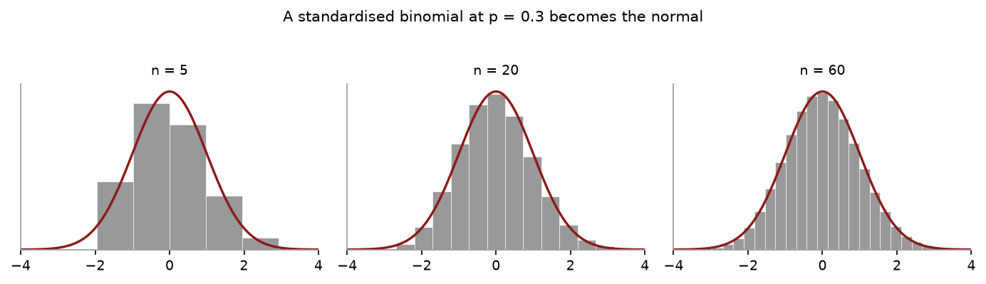
Each panel is an exact binomial at $p = 0.3$, standardised, with the standard normal drawn over it. At $n = 5$ the bars are visibly lumpy and lopsided; by $n = 20$ they have nearly settled; by $n = 60$ you cannot separate them by eye.
import numpy as np, matplotlib.pyplot as plt

p, n = 0.3, 60
k = np.arange(n + 1)
mu, sd = n*p, np.sqrt(n*p*(1-p))

plt.bar((k - mu)/sd, stats.binom.pmf(k, n, p)*sd, width=1/sd, color="#999999")
xs = np.linspace(-4, 4, 300)
plt.plot(xs, stats.norm.pdf(xs), color="#8b1a1a", lw=1.6)
plt.show()
Change n and re-run. Then set p = 0.03 and watch it fail — at $np = 1.8$ the
distribution is piled against zero with no room to be symmetric, which is the
$np \geq 5$ condition made visible.
Not checking the four conditions. Especially constant $p$ — sampling without replacement from a small population breaks it.
Confusing $\mathrm{P}(X = k)$ with $\mathrm{P}(X \le k)$. “Exactly”, “at most” and “at least” are three different calculations, and the wording is the only clue.
Dropping the binomial coefficient. Without $\binom{n}{k}$ you have computed the probability of one specific ordering, not of $k$ successes.
Using $\sigma = np(1-p)$. That is the variance. The standard deviation is its square root.
Doing “at least one” the long way. Use the complement.
Mixing up $k$ and $n-k$ in the exponents. The power on $p$ is the number of successes.
$X \sim \text{Bin}(12, 0.25)$. (a) Find $\mathrm{P}(X = 3)$. (b) Find $E(X)$ and $\sigma$. (c) Is $\mathrm{P}(X = 3)$ the most likely single outcome? Explain without computing every probability.
A multiple-choice quiz has 20 questions, each with four options. A student guesses every one. (a) What are $n$ and $p$? (b) How many would you expect them to get right? (c) Find the standard deviation.
A machine produces items with a 4% defect rate. Six are drawn independently. Find the probability that at least one is defective.
For each, say whether the binomial applies, and if not which condition fails. (a) Number of heads in 50 flips of a fair coin. (b) Number of aces in 5 cards dealt from a 52-card deck. (c) Number of customers arriving at a shop between 9 and 10 am. (d) Number of left-handed people in a random sample of 200 from a city.
$X \sim \text{Bin}(n, 0.5)$ has standard deviation 3. Find $n$.
(a) $\binom{12}{3}(0.25)^3(0.75)^9 = 220 \times 0.015625 \times 0.0750847 = 0.2581$. (b) $E(X) = 12(0.25) = 3$ and $\sigma = \sqrt{12(0.25)(0.75)} = \sqrt{2.25} = 1.5$. (c) Yes. The distribution peaks at or next to $np = 3$, and since $np$ is a whole number here the mode is exactly 3.
(a) $n = 20$, $p = 0.25$. (b) $E(X) = 20(0.25) = 5$. (c) $\sigma = \sqrt{20(0.25)(0.75)} = \sqrt{3.75} = 1.9365$.
$\mathrm{P}(X \ge 1) = 1 - (0.96)^6 = 1 - 0.7828 = 0.2172$.
(a) Yes — all four hold. (b) No. Cards are dealt without replacement, so $p$ changes between draws, and 5 of 52 is nearly 10% of the population, too large for the approximation. (c) No. There is no fixed number of trials — $n$ is not decided in advance. This is a counting-over-time problem, which needs a different distribution. (d) Yes, effectively. Strictly it is without replacement, but 200 from a city is a tiny fraction of the population, so $p$ is constant to any accuracy that matters.
$\sigma^2 = n(0.5)(0.5) = 0.25n = 9$, so $n = 36$.
Ten more. Work questions 1 and 2 with the formula rather than Stata — the exam has no Stata in it, and the only way the factorials stop being frightening is repetition.
A supplier’s components are faulty 25% of the time, independently. Twelve are installed. (a) Check each of the four binomial conditions against this scenario. (b) Find $E(X)$, $V(X)$ and the standard deviation of the number faulty. (c) Find $\mathrm{P}(X = 3)$.
For the same twelve components: (a) Find $\mathrm{P}(X = 0)$. (b) Find $\mathrm{P}(X \geq 1)$, and say which rule saved you most of the work. (c) Find $\mathrm{P}(X \leq 2)$.
A call centre’s lines fail to connect 10% of the time. Twenty calls are placed. (a) Find the probability exactly two fail. (b) Find the probability at least three fail.
For each scenario, say whether the binomial applies, and if not, which condition fails. (a) Counting heads in 50 tosses of a fair coin. (b) Drawing 5 cards from a deck and counting hearts. (c) Counting how many of 30 students pass, when they studied together. (d) Counting the number of customers arriving in an hour. (e) Counting defectives in a sample of 20 from a batch of 10,000 that is 3% defective.
Explain why $\mathrm{P}(X \geq 1) = 1 - \mathrm{P}(X = 0)$ saves so much work, and write down a question for which the complement rule would not help.
For each, say whether the normal approximation to the binomial is appropriate. (a) $n = 40$, $p = 0.5$. (b) $n = 40$, $p = 0.08$. (c) $n = 200$, $p = 0.02$. (d) $n = 15$, $p = 0.6$.
A batch of 10,000 items is 3% defective, and 20 are sampled without replacement. (a) Strictly, is this binomial? (b) Why is treating it as binomial nevertheless fine here? (c) At what sample size would you start to worry?
A basketball player makes 80% of free throws. In a game they take 10. (a) Find the expected number made. (b) Find $\mathrm{P}(\text{all } 10)$. (c) The commentator says “they make 8 out of 10, so expect exactly 8 tonight.” What is wrong with that?
$X \sim \text{Bin}(n, 0.4)$. Write $E(X)$ and $\text{SD}(X)$ as functions of $n$, and say which grows faster as $n$ increases. What does that imply about $X/n$?
A table gives cumulative binomial probabilities $\mathrm{P}(X \leq x)$. Write down, in terms of table entries, how you would get (a) $\mathrm{P}(X = 4)$, (b) $\mathrm{P}(X \geq 4)$, (c) $\mathrm{P}(2 \leq X \leq 5)$.
(a) Fixed $n$: 12 components, decided in advance. Two outcomes: faulty or not. Constant $p$: 0.25 for each, which the question asserts. Independence: stated. All four hold, so $X \sim \text{Bin}(12, 0.25)$. (b) $E(X) = 12(0.25) = 3.0000$; $V(X) = 12(0.25)(0.75) = 2.2500$; $\text{SD}(X) = 1.5000$. (c) $\mathrm{P}(X=3) = \binom{12}{3}(0.25)^3(0.75)^9 = 220(0.015625)(0.0750847) = 0.2581$.
(a) $\mathrm{P}(X=0) = (0.75)^{12} = 0.0317$. (b) $1 - 0.0317 = 0.9683$. The complement rule — the alternative is adding twelve separate terms. (c) $\mathrm{P}(X \leq 2) = 0.0317 + 0.1267 + 0.2323 = 0.3907$.
(a) $\binom{20}{2}(0.1)^2(0.9)^{18} = 190(0.01)(0.1500946) = 0.2852$. (b) $\mathrm{P}(X \geq 3) = 1 - \mathrm{P}(X \leq 2) = 1 - (0.1216 + 0.2702 + 0.2852) = 1 - 0.6769 = 0.3231$.
(a) Yes. (b) No — drawing without replacement from 52 cards changes $p$ between draws, so the constant-$p$ and independence conditions fail. This is hypergeometric. (c) No — studying together breaks independence; one student’s outcome carries information about another’s. (d) No — there is no fixed $n$; arrivals in a fixed period is a Poisson situation. (e) Yes in practice — see question 7.
Because “at least one” is the union of every outcome from 1 to $n$, while its complement is the single outcome 0. One term replaces $n$ of them, and the single term is the easiest one in the distribution, being just $(1-p)^n$. The rule does not help for something like $\mathrm{P}(3 \leq X \leq 7)$, whose complement is two separate tails and therefore no simpler than the original — there you add the five terms, or use cumulative values.
The condition is $np \geq 5$ and $n(1-p) \geq 5$. (a) $np = 20$, $n(1-p) = 20$. Yes. (b) $np = 3.2$. No — fails on the left even though $n(1-p) = 36.8$ passes. (c) $np = 4$. No, and only just: $n = 250$ would do it. (d) $np = 9$, $n(1-p) = 6$. Yes, if marginally.
(a) No. Sampling without replacement means $p$ changes from draw to draw, so strictly this is hypergeometric. (b) Because the batch is enormous relative to the sample. Removing one item from 10,000 moves the defect rate from 0.0300 to roughly 0.0300 — the change is in the fifth decimal place, so the draws are independent for every practical purpose. (c) The usual rule of thumb is when the sample exceeds 5% of the population. Here that is 500 items; at 20 you are nowhere near it.
(a) $10(0.8) = 8.0000$. (b) $0.8^{10} = 0.1074$. (c) The expected value is an average over many games, not a prediction for one. $\mathrm{P}(X = 8)$ is only $\binom{10}{8}(0.8)^8(0.2)^2 = 0.3020$, so the single most likely outcome happens under a third of the time and the other two-thirds of games land somewhere else. “Expect 8” is right about the long-run mean and wrong about tonight.
$E(X) = 0.4n$ and $\text{SD}(X) = \sqrt{0.24n}$. The mean grows linearly in $n$; the standard deviation grows only as $\sqrt{n}$. So the proportion $X/n$ has mean 0.4 fixed and standard deviation $\sqrt{0.24/n}$, which shrinks towards zero. The count becomes more variable in absolute terms and the proportion becomes less variable — which is the whole of Chapter 11 showing up early.
(a) $\mathrm{P}(X \leq 4) - \mathrm{P}(X \leq 3)$. (b) $1 - \mathrm{P}(X \leq 3)$ — note the 3, not the 4; “at least 4” excludes only 0 through 3, and using $\mathrm{P}(X \leq 4)$ here is the commonest table mistake in the chapter. (c) $\mathrm{P}(X \leq 5) - \mathrm{P}(X \leq 1)$.