The question: what changes when the variable can take any value in an interval?
For a discrete variable you add probabilities. For a continuous one you cannot, and the reason is worth seeing rather than memorising.
Ask for the probability that a delivery takes exactly 3 minutes. Not 3.0001, not 2.9999 — exactly 3, to infinite precision. There are infinitely many values it could take, so any single one gets probability
\[\mathrm{P}(X = a) = 0\]That is not a technicality to wave past. It has three consequences you will use.
Only intervals carry probability. $\mathrm{P}(2 < X < 4)$ is a sensible question; $\mathrm{P}(X = 3)$ is not.
Probability is area. The curve is a probability density function, and $\mathrm{P}(a < X < b)$ is the area under it between $a$ and $b$. Total area is 1.
Strict and weak inequalities are the same. $\mathrm{P}(X < a) = \mathrm{P}(X \le a)$, because the endpoint contributes nothing. This is false for discrete variables, and confusing the two cases is a standard exam trap.
One more thing: a density is not a probability, and its height can exceed 1. A uniform distribution on $[0, 0.5]$ has height 2 everywhere. What cannot exceed 1 is the area.
The simplest case: every value in $[a, b]$ is equally likely. The density is a flat line of height $1/(b-a)$, and probabilities are rectangles.
\[\mathrm{P}(c < X < d) = \frac{d - c}{b - a} \qquad \mu = \frac{a+b}{2} \qquad \sigma = \frac{b-a}{\sqrt{12}}\]Example. Delivery times are uniform between 10 and 50 minutes.
\[\mu = \frac{10+50}{2} = 30 \qquad \sigma = \frac{40}{\sqrt{12}} = 11.547 \qquad \mathrm{P}(X < 25) = \frac{25-10}{40} = 0.375\]No tables, no standardising — just the fraction of the interval you want. The uniform is genuinely as simple as it looks, which is why it gets one page.
The bell. Symmetric about $\mu$, with $\sigma$ controlling how wide. Two parameters and you have the whole curve.
It matters for two quite different reasons. Many measured quantities happen to be roughly bell-shaped — and, far more importantly, Chapter 12 will show that sample means are normal whatever the population looks like. Most of the normal’s work in this course is done on behalf of $\bar{X}$, not on behalf of raw data.
There are infinitely many normal curves, one for each $(\mu, \sigma)$, and nobody tabulates them all. Instead, convert to the one that is tabulated:
\[Z = \frac{X - \mu}{\sigma} \sim N(0, 1)\]Chapter 3’s $z$-score, doing a new job. Subtracting $\mu$ centres the curve on zero; dividing by $\sigma$ sets its width to 1.
Always sketch first. Draw the bell, mark $\mu$, mark your value, shade what the question asks for. Then compute. It takes five seconds and it prevents the most common error in this chapter, which is finding the area on the wrong side.
Placement test scores are normal with $\mu = 72$ and $\sigma = 8$.
(a) What proportion score above 80?
\[z = \frac{80-72}{8} = 1.00 \qquad \mathrm{P}(X > 80) = \mathrm{P}(Z > 1) = 1 - 0.8413 = 0.1587\](b) What proportion score between 64 and 80?
Those are $z = -1$ and $z = +1$:
\[\mathrm{P}(-1 < Z < 1) = 0.8413 - 0.1587 = 0.6827\]The familiar 68% from the empirical rule, now derived rather than quoted.
(c) Above what score do the top 10% fall?
This is the table read backwards — you are given an area and want a value. The top 10% begins at $z = 1.2816$, so
\[x = \mu + z\sigma = 72 + 1.2816(8) = 82.25\]Both directions matter and the second is the one students practise less. Given a probability, find $z$ first, then unstandardise with $x = \mu + z\sigma$.
Waiting time until the next event, when events arrive at a constant average rate. Calls to a switchboard, time between machine breakdowns, time until a component fails.
If the mean waiting time is $\mu$, then
\[\mathrm{P}(X > x) = e^{-x/\mu} \qquad \mathrm{P}(X < x) = 1 - e^{-x/\mu} \qquad \sigma = \mu\]That last identity is not a misprint: for an exponential, the standard deviation equals the mean. It is a strongly right-skewed distribution — many short waits, a few very long ones.
Example. Time between arrivals at a service desk averages 4 minutes.
\[\mathrm{P}(X > 6) = e^{-6/4} = e^{-1.5} = 0.2231 \qquad \mathrm{P}(X < 2) = 1 - e^{-2/4} = 1 - 0.6065 = 0.3935\]No table needed — just the exponential function.
| Distribution | Reach for it when |
|---|---|
| Uniform | every value in a range is equally likely |
| Normal | symmetric and bell-shaped — and for sample means, always |
| Exponential | waiting time until the next event |
The snippets below assume the header and preamble from Chapter 1 — clear all, the log, and a cd to your own folder.
The two normal functions, and the fact that they invert each other:
* value -> probability.  normal(z) gives the area to the LEFT.
display "P(X>80)    = " 1 - normal((80-72)/8)
display "P(64<X<80) = " normal((80-72)/8) - normal((64-72)/8)

* probability -> value.  invnormal() takes the area to the left.
display "z for top 10% = " invnormal(0.90)
display "the score     = " 72 + invnormal(0.90)*8
normal() and invnormal() are inverses, which is worth confirming once:
display normal(invnormal(0.90))
For the exponential, no special function is needed:
display "P(X>6) = " exp(-6/4)
display "P(X<2) = " 1 - exp(-2/4)
And to generate continuous data to experiment on:
clear
set seed 250
set obs 10000
generate double y = rnormal(72, 8)
generate double u = runiform(10, 50)
summarize y u
histogram y, normal
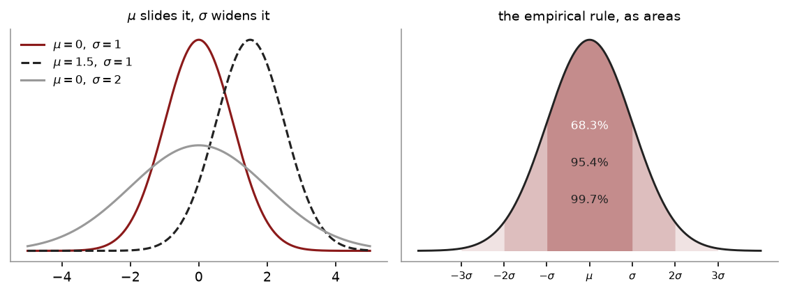
The formula for the normal density is unpleasant and you are never asked to use it. What you do need is a feel for what the two parameters do and what the areas look like, and a picture settles both in seconds.
The left panel is the whole definition. $\mu$ slides the curve left or right without changing its shape; $\sigma$ widens or narrows it without moving its centre. Those are the only two things you can change, which is why naming $\mu$ and $\sigma$ names the entire distribution.
The right panel is the empirical rule drawn as areas rather than quoted as a rule: 68.3% within one standard deviation, 95.4% within two, 99.7% within three.
Change the parameters and re-run:
MU, SIGMA = 72, 8        # <-- change these

import numpy as np
import matplotlib.pyplot as plt
from scipy import stats

xs = np.linspace(MU - 4*SIGMA, MU + 4*SIGMA, 600)
plt.plot(xs, stats.norm.pdf(xs, MU, SIGMA), color="#8b1a1a", lw=1.8)

for k in (1, 2, 3):                       # shade one, two, three sigma
    m = (xs >= MU - k*SIGMA) & (xs <= MU + k*SIGMA)
    plt.fill_between(xs[m], stats.norm.pdf(xs[m], MU, SIGMA),
                     color="#8b1a1a", alpha=0.12, linewidth=0)
    pct = stats.norm.cdf(k) - stats.norm.cdf(-k)
    print(f"within {k} sigma: {pct:.4f}")

plt.yticks([]); plt.show()
Notice the printed percentages do not change when you change MU and SIGMA.
That is the point of standardising: every normal is the same curve in different units.
Chapter 9’s worked example, done both ways. sf is the survival function — the area
to the right — so you never have to subtract from 1:
mu, sigma = 72, 8

# value -> probability
print(stats.norm.sf(80, mu, sigma))                  # P(X > 80)   = 0.1587
print(stats.norm.cdf(80, mu, sigma)
      - stats.norm.cdf(64, mu, sigma))               # P(64<X<80)  = 0.6827

# probability -> value
print(stats.norm.ppf(0.90, mu, sigma))               # top 10% start at 82.25
ppf is the inverse — Stata’s invnormal(). The two are exact inverses, which is worth
confirming once: stats.norm.cdf(stats.norm.ppf(0.9)) returns 0.9.
| Stata | Python |
|---|---|
normal(z) |
stats.norm.cdf(z) |
1 - normal(z) |
stats.norm.sf(z) |
invnormal(p) |
stats.norm.ppf(p) |
display exp(-6/4) |
stats.expon.sf(6, scale=4) |
runiform(10, 50) |
rng.uniform(10, 50, size) |
rnormal(72, 8) |
rng.normal(72, 8, size) |
Python is not taught and not examined in this course — your problem sets are done in Stata. It is here because seeing the same operation written twice is a cheap way to notice which part is the statistics and which part is the software.
Looking for $\mathrm{P}(X = a)$ on a continuous variable. It is zero. The question must mean an interval.
Finding the area on the wrong side. normal() and most printed tables give the area
to the left. For an upper tail, subtract from 1. Sketching prevents this.
Forgetting to unstandardise. When the question asks for a score and you have found $z = 1.2816$, you are not finished: $x = \mu + z\sigma$.
Using $\sigma^2$ where $\sigma$ belongs. $N(72, 64)$ and $N(72, 8)$ describe the same distribution under different conventions — check whether you have been given the variance or the standard deviation.
Treating a density height as a probability. It can exceed 1; only area cannot.
$X \sim N(100, 15^2)$. (a) Find $\mathrm{P}(X > 120)$. (b) Find $\mathrm{P}(85 < X < 130)$. (c) Below what value do the bottom 5% fall?
Waiting times at a counter are uniform between 0 and 12 minutes. (a) Find the mean and standard deviation. (b) Find $\mathrm{P}(X > 9)$. (c) Find $\mathrm{P}(3 < X < 7)$.
The time between breakdowns of a machine is exponential with a mean of 20 days. (a) Find the probability it runs more than 30 days without breaking down. (b) Find the probability it breaks down within the first week. (c) What is the standard deviation?
A classmate writes $\mathrm{P}(X = 50) = 0.04$ for a continuous variable. Explain what has gone wrong and what they probably meant.
Scores are normal with $\mu = 500$ and $\sigma = 100$. A scholarship goes to the top 2.5%. What is the cut-off, and what $z$ did you use?
(a) $z = (120-100)/15 = 1.3333$, so $\mathrm{P} = 1 - 0.9088 = 0.0912$. (b) $z = -1$ and $z = 2$, so $0.9772 - 0.1587 = 0.8186$. (c) $z = -1.6449$, so $x = 100 - 1.6449(15) = 75.33$.
(a) $\mu = 6$; $\sigma = 12/\sqrt{12} = 3.4641$. (b) $(12-9)/12 = 0.25$. (c) $(7-3)/12 = 0.3333$.
(a) $e^{-30/20} = e^{-1.5} = 0.2231$. (b) $1 - e^{-7/20} = 1 - 0.7047 = 0.2953$. (c) 20 days — for an exponential, the standard deviation equals the mean.
For a continuous variable the probability of any exact value is zero, so $\mathrm{P}(X=50)$ cannot be 0.04. They have most likely computed the density at 50, which is a height and not a probability, or they meant an interval around 50 such as $\mathrm{P}(49.5 < X < 50.5)$.
The top 2.5% starts at $z = 1.96$, so the cut-off is $500 + 1.96(100) = 696$.
Ten more, across all three distributions. Draw the picture first every single time — every mistake in this chapter is a shaded region on the wrong side of a line, and a sketch costs ten seconds.
Waiting time at a service desk is uniform on $[10, 50]$ minutes. (a) Find the mean, variance and standard deviation. (b) Find $\mathrm{P}(X < 25)$. (c) Find $\mathrm{P}(20 < X < 35)$. (d) Find $\mathrm{P}(X = 25)$, and explain the answer.
Test scores are $N(500, 100^2)$. (a) Find $\mathrm{P}(X > 650)$. (b) Find $\mathrm{P}(400 < X < 600)$. (c) Find $\mathrm{P}(X < 430)$. (d) Find the 90th percentile.
For the same distribution, a scholarship goes to the top 5%. What is the cut-off, and which direction does the $z$ run?
The time between arrivals at a till is exponential with a mean of 8 minutes. (a) Find $\lambda$ and the standard deviation. (b) Find $\mathrm{P}(X > 10)$. (c) Find $\mathrm{P}(X < 5)$. (d) Find the median waiting time, and say why it is not 8.
For the same arrivals: five minutes have passed with no one arriving. Find the probability you wait at least ten more. Compare it with your answer to 4(b) and name the property.
Explain why $\mathrm{P}(X = c) = 0$ for any continuous random variable, and why this does not mean the value $c$ is impossible.
For each quantity, name the distribution you would reach for first and say what feature of the situation decides it. (a) The height of adult women. (b) The time until a lightbulb fails. (c) A random number generated between 0 and 1. (d) The sum of 40 small independent shocks. (e) The time between emails arriving.
A process is $N(\mu, \sigma^2)$ and 2.5% of output falls below 46 while 2.5% falls above 74. Find $\mu$ and $\sigma$ without using a single probability table entry beyond $z = 1.96$.
A student computes $z = (430 - 500)/100 = -0.70$ and reports $\mathrm{P}(X < 430) = 0.7580$. Identify the error and give the correct answer.
Scores are $N(500, 100^2)$. Explain why $\mathrm{P}(X > 650)$ and $\mathrm{P}(\bar{X} > 650)$ for a sample of 25 are wildly different numbers, without computing the second one.
(a) Mean $= (10+50)/2 = 30.0000$; $V = (50-10)^2/12 = 1600/12 = 133.3333$; SD $= 11.5470$. (b) The density is $1/40$ throughout, so the probability is the width over the range: $(25-10)/40 = 0.3750$. (c) $(35-20)/40 = 0.3750$ — the same answer, because the interval has the same width. Under a uniform, only the width matters, never the location. (d) Zero. A single point has no width, and probability is area. See question 6.
(a) $z = (650-500)/100 = 1.50$, so $\mathrm{P} = 0.0668$. (b) $z = \pm 1.00$, so $\mathrm{P} = 0.6827$ — the familiar 68%. (c) $z = -0.70$, so $\mathrm{P} = 0.2420$. (d) $z_{0.90} = 1.2816$, so the 90th percentile is $500 + 1.2816(100) = 628.1552$.
The top 5% means 5% in the upper tail, so $z = +1.6449$ and the cut-off is $500 + 1.6449(100) = 664.4854$. The sign is the thing to get right: a cut-off above the mean must have a positive $z$, and if your arithmetic returns something below 500 you have used $-1.6449$ by mistake.
(a) $\lambda = 1/8 = 0.1250$ per minute. For an exponential the standard deviation equals the mean, so SD $= 8.0000$ minutes. (b) $\mathrm{P}(X > 10) = e^{-10/8} = e^{-1.25} = 0.2865$. (c) $\mathrm{P}(X < 5) = 1 - e^{-5/8} = 1 - 0.5353 = 0.4647$. (d) The median solves $e^{-\lambda m} = 0.5$, giving $m = \ln 2/\lambda = 0.6931 \times 8 = 5.5452$ minutes. It is below the mean because the exponential is strongly right-skewed — most waits are short and a few very long ones drag the mean up past the middle.
$\mathrm{P}(X > 15 \mid X > 5) = e^{-10/8} = 0.2865$, identical to 4(b). This is the memoryless property: the distribution of the remaining wait does not depend on how long you have already waited. It is the defining feature of the exponential and the reason it describes arrivals that have no pattern — the process does not know you are standing there.
Probability is the area under the density, and the area above a single point is a rectangle of zero width, hence zero. It does not mean $c$ is impossible, because every value has probability zero and yet one of them occurs. For a continuous variable, zero probability and impossibility are different things — which is why continuous questions are always asked about intervals, and why it makes no difference whether you write $<$ or $\leq$.
(a) Normal — a quantity built from many small additive influences. (b) Exponential — a waiting time with a constant failure rate. (c) Uniform — every value in the range equally likely by construction. (d) Normal, by the CLT — the giveaway is the word “sum”. (e) Exponential — a gap between events in a memoryless process.
The two cut-offs are symmetric about the mean, so $\mu = (46 + 74)/2 = 60.0000$. Each is 14 away from the mean and sits at $z = \pm 1.96$, so $1.96\sigma = 14$ and $\sigma = 14/1.96 = 7.1429$. Reading a normal problem backwards like this — from the tails to the parameters — is exactly what confidence intervals will ask you to do in Chapter 13.
The $z$ is right and the probability is the complement of the answer. The student has looked up $\mathrm{P}(Z < 0.70) = 0.7580$, dropping the minus sign. For a negative $z$ the lower-tail area must be below 0.5, so 0.7580 should have been rejected on sight. The correct answer is $\mathrm{P}(Z < -0.70) = 0.2420$, and $0.2420 + 0.7580 = 1$ confirms the relationship between the two.
Because the two questions are about different random variables. A single score has standard deviation 100, so 650 is 1.5 standard deviations out — unusual but ordinary. A sample mean of 25 scores has standard error $100/\sqrt{25} = 20$, so 650 is seven and a half standard errors out. Averaging destroys the extremes: for the mean of 25 students to exceed 650, essentially all of them have to be exceptional at once, and that is enormously rarer than one student being so.