The question: the normal needs $\sigma$. What do you use when you have to estimate it?
These three arrive together and look like three new table formats to memorise. They are not. Each is built out of standard normals, and if you can say what each is made of, you can work out what it is for.
| Built from | About | |
|---|---|---|
| $\chi^2_\nu$ | $Z_1^2 + Z_2^2 + \cdots + Z_\nu^2$ — standard normals squared and added | one variance |
| $t_\nu$ | a $Z$ divided by $\sqrt{\chi^2_\nu/\nu}$ — a normal over an estimated spread | a mean, when $\sigma$ is unknown |
| $F_{\nu_1,\nu_2}$ | $\dfrac{\chi^2{\nu_1}/\nu_1}{\chi^2{\nu_2}/\nu_2}$ — a ratio of two $\chi^2$s | comparing two variances |
Everything below is commentary on that table.
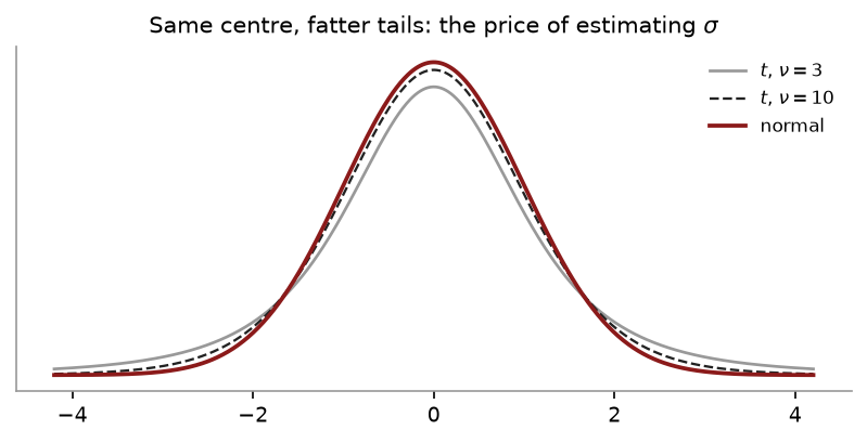
Same bell shape as the normal, centred at zero, but with fatter tails. One parameter: the degrees of freedom $\nu$, which in this course is almost always $n - 1$ — the same $n-1$ from Chapter 3.
Here is the whole argument, and it is worth getting rather than accepting.
\[z = \frac{\bar{x} - \mu}{\sigma/\sqrt{n}} \qquad\text{against}\qquad t = \frac{\bar{x} - \mu}{s/\sqrt{n}}\]In $z$, the denominator is a fixed number. In $t$, it is $s$, which is computed from the same sample and therefore jumps around. Two sources of randomness instead of one.
And the damage is asymmetric. When $s$ happens to come out small, the ratio blows up. With only five observations, $s$ lands below $0.7\sigma$ about a quarter of the time — so “blows up” is not a rare accident, it is a quarter of your samples.
A simulation makes it concrete. Drawing 1,000 samples from a normal population at $n = 5$:
| share beyond 1.96 | |
|---|---|
| $\lvert z\rvert$ | 0.045 — the 5% the normal table promises |
| $\lvert t\rvert$ | 0.116 — more than double |
Use the normal’s critical value on a $t$ statistic at $n = 5$ and you reject nearly three times too often.
As $\nu$ grows, $s$ settles down towards $\sigma$ and the surcharge shrinks:
| $\nu$ | $t_{0.025,\nu}$ | against $z = 1.96$ |
|---|---|---|
| 4 | 2.7764 | 42% larger |
| 10 | 2.2281 | 14% |
| 30 | 2.0423 | 4% |
| 100 | 1.9840 | 1% |
| $\infty$ | 1.9600 | — |
The bottom row is the normal. That is the real content of the “use $z$ for large samples” rule of thumb.
It is not “a standard error in the denominator means $t$.”
The question is whether the denominator is known or estimated from the same data.
$\dfrac{\bar{x}-\mu}{\sigma/\sqrt{n}}$ — $\sigma$ handed to you. This is $z$, and $\sigma/\sqrt{n}$ is still called the standard error.
$\dfrac{\bar{x}-\mu}{s/\sqrt{n}}$ — you computed $s$. This is $t$.
The counterexample that settles it: tests about proportions use an estimated standard error and still use $z$.
$\chi^2_\nu$ is a sum of $\nu$ squared standard normals. Two consequences fall straight out of that, and you should be able to recite them:
It cannot be negative. It is a sum of squares.
It is right-skewed. Squaring stretches the large values and compresses the small ones.
Because it is not symmetric, there is no trick for getting the lower tail from the upper one — check which tail your table gives you. As $\nu$ grows it becomes more symmetric, for the reason you would now guess: it is a sum, and sums go normal.
It is also built for exactly one job: adding up squared errors. Take your data, subtract what your model predicted, square each gap, add them. That sum is a $\chi^2$, which is why the same distribution reappears when we test categorical data later in the course.
$F$ is one $\chi^2$ divided by another, each first divided by its own degrees of freedom. So it is also non-negative and right-skewed, and it needs two degrees of freedom — numerator first, always.
\[F_{\nu_1,\nu_2} \neq F_{\nu_2,\nu_1}\]Getting the order backwards is the characteristic $F$ error.
Reading it: an $F$ near 1 says the two variances look alike. A large $F$ says the numerator group is much more spread out.
| You need | Worked value | |
|---|---|---|
| $t$ | $\nu$ and a tail area | $\nu = 10$, 2.5% above $\Rightarrow$ 2.2281 |
| $\chi^2$ | $\nu$ and a tail area | $\nu = 10$, 5% above $\Rightarrow$ 18.3070 |
| $F$ | two $\nu$s and a tail | $\nu_1 = 5$, $\nu_2 = 10$, 5% above $\Rightarrow$ 3.3258 |
$t$ is symmetric, so one column serves both tails. $\chi^2$ and $F$ are not, so read the heading.
This is the question that comes up every year, and it is a good question rather than a confused one:
The $z$ table is full of numbers between 0 and 1. The $t$ table is full of numbers bigger than 1. Where is the probability?
The observation is exactly right, and it is the answer. A probability can never be bigger than 1. So the moment every entry in the body of the $t$ table exceeds 1, you know the body is not probabilities. It is something else.
The two tables are built inside out from each other:
| You go in with | You read out | |
|---|---|---|
| $z$ table | a $z$-score | an area — a probability in $[0,1]$ |
| $t$ table | $\nu$ and a tail area | a cutoff — a value of $t$ |
On the $z$ table the probabilities are in the body. On the $t$ table the probabilities are the column headings, and they are the only probabilities on the page. Everything in the body is a $t$ statistic.
So the $t$ table is a critical value table. It answers where is the line?, not how far past it did I land? Said in one sentence, which is worth memorising:
The $z$ table has probabilities inside and $z$-scores on the edges. The $t$ table has $t$-scores inside and probabilities on the edges.
Column headings are the area in the upper tail. For a two-tailed test at $\alpha$, read the $\alpha/2$ column — so a 95% interval uses the 0.025 column, not the 0.05 one. The $\nu = \infty$ row is the standard normal, which is why the “use $z$ when $n$ is large” rule works.
| $\nu$ | 0.10 | 0.05 | 0.025 | 0.01 | 0.005 |
|---|---|---|---|---|---|
| 1 | 3.0777 | 6.3138 | 12.7062 | 31.8205 | 63.6567 |
| 2 | 1.8856 | 2.9200 | 4.3027 | 6.9646 | 9.9248 |
| 3 | 1.6377 | 2.3534 | 3.1824 | 4.5407 | 5.8409 |
| 4 | 1.5332 | 2.1318 | 2.7764 | 3.7469 | 4.6041 |
| 5 | 1.4759 | 2.0150 | 2.5706 | 3.3649 | 4.0321 |
| 6 | 1.4398 | 1.9432 | 2.4469 | 3.1427 | 3.7074 |
| 7 | 1.4149 | 1.8946 | 2.3646 | 2.9980 | 3.4995 |
| 8 | 1.3968 | 1.8595 | 2.3060 | 2.8965 | 3.3554 |
| 9 | 1.3830 | 1.8331 | 2.2622 | 2.8214 | 3.2498 |
| 10 | 1.3722 | 1.8125 | 2.2281 | 2.7638 | 3.1693 |
| 11 | 1.3634 | 1.7959 | 2.2010 | 2.7181 | 3.1058 |
| 12 | 1.3562 | 1.7823 | 2.1788 | 2.6810 | 3.0545 |
| 13 | 1.3502 | 1.7709 | 2.1604 | 2.6503 | 3.0123 |
| 14 | 1.3450 | 1.7613 | 2.1448 | 2.6245 | 2.9768 |
| 15 | 1.3406 | 1.7531 | 2.1314 | 2.6025 | 2.9467 |
| 16 | 1.3368 | 1.7459 | 2.1199 | 2.5835 | 2.9208 |
| 17 | 1.3334 | 1.7396 | 2.1098 | 2.5669 | 2.8982 |
| 18 | 1.3304 | 1.7341 | 2.1009 | 2.5524 | 2.8784 |
| 19 | 1.3277 | 1.7291 | 2.0930 | 2.5395 | 2.8609 |
| 20 | 1.3253 | 1.7247 | 2.0860 | 2.5280 | 2.8453 |
| 21 | 1.3232 | 1.7207 | 2.0796 | 2.5176 | 2.8314 |
| 22 | 1.3212 | 1.7171 | 2.0739 | 2.5083 | 2.8188 |
| 23 | 1.3195 | 1.7139 | 2.0687 | 2.4999 | 2.8073 |
| 24 | 1.3178 | 1.7109 | 2.0639 | 2.4922 | 2.7969 |
| 25 | 1.3163 | 1.7081 | 2.0595 | 2.4851 | 2.7874 |
| 26 | 1.3150 | 1.7056 | 2.0555 | 2.4786 | 2.7787 |
| 27 | 1.3137 | 1.7033 | 2.0518 | 2.4727 | 2.7707 |
| 28 | 1.3125 | 1.7011 | 2.0484 | 2.4671 | 2.7633 |
| 29 | 1.3114 | 1.6991 | 2.0452 | 2.4620 | 2.7564 |
| 30 | 1.3104 | 1.6973 | 2.0423 | 2.4573 | 2.7500 |
| 35 | 1.3062 | 1.6896 | 2.0301 | 2.4377 | 2.7238 |
| 40 | 1.3031 | 1.6839 | 2.0211 | 2.4233 | 2.7045 |
| 50 | 1.2987 | 1.6759 | 2.0086 | 2.4033 | 2.6778 |
| 60 | 1.2958 | 1.6706 | 2.0003 | 2.3901 | 2.6603 |
| 80 | 1.2922 | 1.6641 | 1.9901 | 2.3739 | 2.6387 |
| 100 | 1.2901 | 1.6602 | 1.9840 | 2.3642 | 2.6259 |
| 120 | 1.2886 | 1.6577 | 1.9799 | 2.3578 | 2.6174 |
| $\infty$ | 1.2816 | 1.6449 | 1.9600 | 2.3263 | 2.5758 |
You cannot read an exact $p$-value off this table, because your $t$ will almost never be one of the five numbers in its row. What you can do is bracket it: find $|t|$ in the $\nu$ row, see which two columns it falls between, and read off the areas either side.
Take $t = 3.2$ with $\nu = 24$ — the invoice question from Chapter 14. The row reads
\[1.3178 \quad 1.7109 \quad 2.0639 \quad 2.4922 \quad 2.7969\]and $3.2$ is past the last of them. So it is off the end of the table, and the most the table can say is
\[\text{one tail: } p < 0.005 \qquad\qquad \text{two tails: } p < 0.01\]That is a complete answer. Write “$p < 0.01$, so reject at the 5% level”. The exact value is $0.0038$, so the table was right — just coarse.
The more usual case lands in the middle. For $t = 2.2$ with $\nu = 24$, we have $2.0639 < 2.2 < 2.4922$, so $t$ sits between the 0.025 column and the 0.01 column:
\[\text{one tail: } 0.01 < p < 0.025 \qquad\qquad \text{two tails: } 0.02 < p < 0.05\]and since the two-tailed $p$ is under 0.05, you reject at 5%. The exact value is $0.0377$, inside the bracket.
The direction reverses, and this is where people slip. A bigger $t$ means a smaller area beyond it. So the column with the larger cutoff gives the smaller $p$. Read the brackets off slowly the first few times.
None of this is a limitation you should resent. If you have fixed $\alpha$ in advance — which you should have — you never needed the exact $p$ at all. You needed to know which side of the line you were on, and that is the one question this table answers perfectly.
The snippets below assume the header and preamble from Chapter 1 — clear all, the log, and a cd to your own folder.
Two families, running in opposite directions, and keeping them straight is most of the skill:
* AREA -> CUTOFF.  These take the area to the LEFT.
display "t,    nu=10, 2.5% above = " invt(10, 0.975)
display "t,    nu=inf (that is z) = " invnormal(0.975)
display "chi2, nu=10, 5% above    = " invchi2(10, 0.95)
display "chi2, nu=10, 5% below    = " invchi2(10, 0.05)
display "F,    5 over 10, 5% above = " invF(5, 10, 0.95)
display "F,    10 over 5, 5% above = " invF(10, 5, 0.95)
Note the last two differ — that is $F_{\nu_1,\nu_2} \neq F_{\nu_2,\nu_1}$ in one line.
* CUTOFF -> AREA.  The tail functions give the area ABOVE.
display "P(t_10 > 2.2281)  = " ttail(10, 2.2281)
display "P(chi2_10 > 18.31) = " chi2tail(10, 18.3070)
display "P(F_5,10 > 3.3258) = " Ftail(5, 10, 3.3258)
invt goes area → cutoff; ttail goes cutoff → area. A critical value is the first
question. A p-value is the second. That distinction is the whole of Chapter 14.
You can also watch the constructions happen:
* a chi-squared really is squared z's added up
clear
set seed 250
set obs 10000
generate double ss = 0
forvalues j = 1/10 {
    quietly generate double z`j' = rnormal()
    quietly replace ss = ss + z`j'^2
}
summarize ss
The mean should come out near 10 — because $E(\chi^2_\nu) = \nu$, which is another fact that falls out of the construction: each $Z^2$ contributes 1 on average.
from scipy import stats

# AREA -> CUTOFF.  ppf takes the area to the LEFT.
stats.t.ppf(0.975, 10)        #  2.2281   invt(10, 0.975)
stats.chi2.ppf(0.95, 10)      # 18.3070   invchi2(10, 0.95)
stats.f.ppf(0.95, 5, 10)      #  3.3258   invF(5, 10, 0.95)
stats.norm.ppf(0.975)         #  1.9600   the t table's infinity row

# CUTOFF -> AREA.  sf is the area to the RIGHT.
stats.t.sf(2.2281, 10)        # 0.0250   ttail(10, 2.2281)
stats.chi2.sf(18.3070, 10)    # 0.0500
stats.f.sf(3.3258, 5, 10)     # 0.0500
ppf and sf are the two directions, and they are exact inverses. A critical value
is ppf; a p-value is sf.
Same centre, same bell shape, heavier tails — and the lower the degrees of freedom the heavier they get. The numbers behind the picture:
for df in (3, 10, 30):
    print(df, 2*stats.t.sf(2, df))     # 0.1393, 0.0734, 0.0578
print("normal", 2*stats.norm.sf(2))    # 0.0455
At $\nu = 3$ a value beyond $\pm 2$ happens three times as often as the normal says. By $\nu = 30$ the gap has nearly closed. That is the surcharge for estimating $\sigma$, shrinking as the sample grows.
import numpy as np
rng = np.random.default_rng(250)

z = rng.normal(size=(100_000, 10))     # ten standard normals, many times
chi = (z**2).sum(axis=1)               # square them and add

print(chi.mean())                      # near 10 -- because E(chi2_v) = v
print((chi > 18.3070).mean())          # near 0.05
Each $Z^2$ contributes 1 on average, which is why the mean is the degrees of freedom. Nothing about the table is needed to see it.
Using $z$ when $\sigma$ was estimated. At large $n$ the numerical difference is cosmetic, but the reasoning is what is being marked.
Getting the degrees of freedom wrong. For a one-sample $t$ it is $n - 1$, not $n$.
Reversing the $F$ degrees of freedom. Numerator first.
Assuming symmetry for $\chi^2$ or $F$. Neither is symmetric, so you cannot flip a sign to get the other tail.
Confusing invt with ttail. One takes an area, the other returns one.
Thinking these are about new situations. They are about the same questions as before — a mean, a variance, two variances — under the realistic condition that you had to estimate something.
Using Stata functions or a table, find: (a) $t_{0.05,\,15}$ (b) $t_{0.025,\,24}$ (c) $\chi^2{0.05,\,8}$ (d) $F{0.05,\,3,\,12}$
Explain, in two sentences and without formulas, why the $t$ distribution has fatter tails than the normal.
A sample of $n = 16$ gives $\bar{x} = 52$ and $s = 8$, and the population mean is claimed to be 48. (a) Should you use $z$ or $t$? Why? (b) How many degrees of freedom? (c) Compute the test statistic.
Why can a $\chi^2$ value never be negative? Answer from the construction, not from a table.
A classmate computes $F_{10,5}$ when the question asked for $F_{5,10}$. Does it matter? Check with Stata or a table and explain.
(a) 1.7531 (b) 2.0639 (c) 15.5073 (d) 3.4903.
In Stata: invt(15,0.95), invt(24,0.975), invchi2(8,0.95), invF(3,12,0.95).
Because $t$ divides by $s$ rather than by $\sigma$, and $s$ is itself random — it changes from sample to sample. When $s$ comes out small the whole ratio is pushed far from zero, so extreme values occur more often than the normal predicts.
(a) $t$ — $\sigma$ is unknown and $s$ was computed from the same 16 observations. (b) $\nu = 15$. (c) SE $= 8/\sqrt{16} = 2$, so $t = (52-48)/2 = 2.00$.
A $\chi^2_\nu$ is the sum of $\nu$ squared standard normals. Every term is a square, so every term is at least zero, so the sum is at least zero. Nothing about the table is needed.
Yes, it matters. $F_{0.05,5,10} = 3.3258$ while $F_{0.05,10,5} = 4.7351$ — not remotely the same. The $F$ is a ratio, and swapping the degrees of freedom swaps which group is on top, which is a different question.
Nine more. These are table-reading drills, and they are worth doing because a test statistic computed perfectly and compared against the wrong critical value scores zero.
Find each critical value. (a) $t_{0.025, 15}$. (b) $t_{0.05, 15}$. (c) $t_{0.025, 24}$. (d) $t_{0.025, 100}$. (e) $z_{0.025}$.
Look at your answers to 1(c), 1(d) and 1(e) together. What is happening as the degrees of freedom rise, and why?
Find each. (a) $\chi^2{0.05, 10}$. (b) $\chi^2{0.95, 10}$. (c) $\chi^2_{0.025, 20}$.
Why does the chi-squared distribution have two different critical values for a two-tailed problem at 5%, when the $t$ has one value used twice?
Find (a) $F_{0.05, 5, 10}$ and (b) $F_{0.05, 10, 5}$. Explain why they differ.
Verify that $\big(t_{0.025, 10}\big)^2 = F_{0.05, 1, 10}$, and explain the relationship between the two distributions that makes this true.
For each situation, name the distribution you would use. (a) Testing a mean with $\sigma$ known. (b) Testing a mean with $\sigma$ estimated from a sample of 18. (c) Testing whether three group means are all equal. (d) Testing whether observed counts match a claimed distribution. (e) Testing a mean with $\sigma$ estimated from a sample of 2,000.
A researcher has $n = 16$ and uses $z = 1.96$ because “the sample is large enough”. (a) What should they have used? (b) By how much is their critical value too small, in percentage terms? (c) Which way does the error push their conclusions?
Explain, in two or three sentences each, where the degrees of freedom come from in (a) a one-sample $t$ test, (b) a chi-squared test on a $3 \times 4$ table, and (c) the numerator of an $F$ test comparing four group means.
(a) 2.1314. (b) 1.7531. (c) 2.0639. (d) 1.9840. (e) 1.9600.
The $t$ critical value is falling towards the $z$ value: 2.0639 at $\nu = 24$, 1.9840 at $\nu = 100$, against 1.9600 for the normal. The $t$ is wider than the normal because $s$ is itself estimated and therefore uncertain, and that extra uncertainty has to be paid for with a longer interval. As $n$ grows, $s$ pins down $\sigma$ more and more tightly, the extra uncertainty vanishes, and the two distributions converge. By $\nu = 100$ the difference is in the second decimal place, which is why people get away with using $z$ — but it is a convenience, not a rule.
(a) 18.3070. (b) 3.9403. (c) 34.1696.
Because the chi-squared distribution is not symmetric. It lives on $[0, \infty)$ and is right-skewed, so the point cutting off 2.5% in the upper tail is not the mirror image of the point cutting off 2.5% in the lower one, and both must be looked up separately. The $t$ is symmetric about zero, so one magnitude serves for both tails with a sign attached.
(a) 3.3258. (b) 4.7351. They differ because $F$ is a ratio of two variance estimates and the two degrees of freedom do different jobs — one describes the numerator, one the denominator. Swapping them is not a relabelling, it is a different distribution, which is why the convention “numerator first” has to be held to.
$t_{0.025, 10} = 2.2281$, and $2.2281^2 = 4.9646$, which is $F_{0.05, 1, 10} = 4.9646$. The reason: a $t$ variable is a standard normal over the square root of a scaled chi-squared, so squaring it gives a chi-squared with 1 degree of freedom over a chi-squared with 10 — and that ratio is precisely an $F$ with $\nu_1 = 1$ and $\nu_2 = 10$. The practical consequence is that a two-tailed $t$ test and an $F$ test on the same single parameter are the same test, which is why a regression’s $t$ on a lone slope and its overall $F$ always agree.
(a) $z$. (b) $t$ with $\nu = 17$. (c) $F$. (d) $\chi^2$. (e) Strictly $t$ with $\nu = 1999$, which to four decimal places is $z$ — but write $t$, because what licenses $z$ is knowing $\sigma$, and a large $n$ only makes the $t$ look like a $z$.
(a) $t_{0.025, 15} = 2.1314$. (b) $(2.1314 - 1.96)/2.1314 = 8.0438\%$ too small. (c) Towards over-rejection. A critical value that is too small makes the rejection region too large, so the researcher rejects null hypotheses more often than their stated 5% allows — their real Type I error rate is above the one they are claiming.
(a) The deviations are taken from $\bar{x}$, which was itself computed from the data. Once $\bar{x}$ and any $n-1$ observations are known, the last one is determined, so only $n-1$ of the deviations are free. One estimated parameter costs one degree of freedom. (b) $(3-1)(4-1) = 6$. With the row and column totals fixed, you can fill in six cells freely and the remaining six are forced by the margins. The margins are not extra information — they are the data’s own totals. (c) $k - 1 = 3$ for four groups. The between-group variation is built from four group means measured against the grand mean, and since the grand mean is a weighted average of those four, knowing three of them and the grand mean fixes the fourth.