The question: Chapter 11 gave you the centre and the spread of $\bar{X}$. What about its shape?
You know $E(\bar{X}) = \mu$ and $\mathrm{SD}(\bar{X}) = \sigma/\sqrt{n}$. Both came out of the rules for expectation and variance in Chapter 7, and both hold for any population whatsoever.
But a centre and a spread are not enough to compute a probability. To say anything like “there is a 5% chance $\bar{X}$ exceeds 19” you need the whole distribution — you need to know which curve to find an area under.
The Central Limit Theorem supplies it, and it supplies it on terms that are almost too generous to believe.
For a random sample of size $n$ drawn from any population with mean $\mu$ and finite standard deviation $\sigma$, the sampling distribution of $\bar{X}$ becomes approximately normal as $n$ grows:
\[\bar{X} \ \dot\sim\ N\!\left(\mu,\ \frac{\sigma^2}{n}\right) \qquad\text{equivalently}\qquad Z = \frac{\bar{X} - \mu}{\sigma/\sqrt{n}} \ \dot\sim\ N(0, 1)\]
Read the word any again. Not “any symmetric population”, not “any population without outliers”. Skewed, bimodal, uniform, discrete — it does not matter. Average enough draws and the average is normal.
That is a genuinely strange result, and it is the reason the normal distribution occupies the place it does in statistics. The normal is not common in nature because of some mysterious preference. It is common because so many of the quantities we measure are secretly averages or sums, and sums of independent things go normal whatever they are sums of.
Take something that is plainly not normal.
A gym weight stack wears unevenly: the middle plates are rubbed shiny and the top and bottom ones stay dusty. Nobody collected that data — hundreds of people independently chose a weight and the metal kept score. The distribution of those choices is lopsided, with a long tail towards the heavy end.
Now change one thing. Suppose every person does six sets and we record each person’s own average. One number per person. Plot those.
| every set everyone did | one average per person | |
|---|---|---|
| $n$ | 1 | 6 |
| standard deviation | 24.1 lb | 9.7 lb |
| shape | skewed right | symmetric |
Three things happened, and each is one of the results you now have.
The spread shrank, from 24.1 to 9.7. That is $\sigma/\sqrt{n}$ with $n = 6$: $24.1/\sqrt{6} = 9.8$. The standard error, measured rather than predicted.
The centre did not move. $E(\bar{X}) = \mu$.
The shape changed. The left panel is skewed. The right panel, built from exactly the same choices, is not. Nobody made the population normal — we took averages, and averages go normal.
There is a matching result for skewness that is worth knowing because it tells you how fast:
\[\text{skewness of } \bar{X} \;=\; \frac{\text{skewness of the population}}{\sqrt{n}}\]The asymmetry does not merely fade, it fades at the same $\sqrt{n}$ rate as the spread.
You will see “$n \geq 30$” quoted as a rule. It is a rule of thumb and not a law, and the honest answer is it depends on how skewed the population is.
Here is the evidence, from a deliberately nasty population — strongly left-skewed, with skewness $-2.11$. For each sample size, 1,000 simulated samples, and we count how many sample means fall below, inside and above the interval the normal approximation predicts should hold 95% of the time:
| $n$ | skewness of $\bar{X}$ | below | inside | above |
|---|---|---|---|---|
| 4 | $-1.05$ | 0.047 | 0.953 | 0.000 |
| 9 | $-0.63$ | 0.049 | 0.942 | 0.009 |
| 36 | $-0.29$ | 0.030 | 0.955 | 0.015 |
| 100 | $-0.34$ | 0.034 | 0.937 | 0.029 |
The skewness column follows the $\sqrt{n}$ prediction closely: $-2.11/\sqrt{4} = -1.06$ against a simulated $-1.05$.
But look at the row for $n = 4$, because it contains a trap.
The “inside” share is 0.953 — almost exactly the 0.95 promised. On that evidence the normal approximation looks perfect. It is not. The two tails are 0.047 and 0.000 against 0.025 each. The left tail is nearly double what it should be and the right tail is empty, and the two errors cancel in the total.
So a two-sided 95% statement survives at $n = 4$ by sheer luck. Any one-tailed probability is badly wrong — $\mathrm{P}(\bar{X} < 1.5)$ would be understated, and an upper-tail probability overstated.
By $n = 36$ both tails are within noise of 0.025. So for a population this skewed, roughly 36 or more, and more again if a one-tailed probability is what you actually care about.
Thirty is a rule of thumb, not a law. For a badly skewed population it is about the minimum; for a symmetric one you can often get away with far less.
You already met a version of this in Chapter 8 without it being called the CLT.
A binomial count is a sum: $X = $ the number of successes in $n$ independent trials is $n$ Bernoulli variables added up. Sums of independent things go normal. So:
\[X \sim \text{Bin}(n, p) \quad\Longrightarrow\quad X \ \dot\sim\ N\big(np,\ np(1-p)\big) \text{ for large } n\]Standardise a binomial at $p = 0.3$ and plot it for $n = 5$, then 20, then 60, and the lumpy, lopsided set of bars at $n = 5$ has nearly settled onto a bell by 20 and is indistinguishable from one by 60.
The usual working condition is $np \geq 5$ and $n(1-p) \geq 5$. Both are needed: at $n = 60$ and $p = 0.01$ you have $np = 0.6$, and the distribution is piled against zero with nowhere to be symmetric.
Daily sales per outlet for a coffee chain have $\mu = 18$ (hundred cups) and $\sigma = 6$. The distribution of individual outlets is right-skewed. A random sample of $n = 36$ outlets is drawn.
(a) What is the distribution of $\bar{X}$?
(b) Find $\mathrm{P}(\bar{X} > 19)$.
(c) Can you find the probability that a single outlet sells more than 19?
(a) By the CLT, $\bar{X}$ is approximately normal with $E(\bar{X}) = 18$ and $\mathrm{SD}(\bar{X}) = 6/\sqrt{36} = 1$.
(b) Standardise:
\[z = \frac{19 - 18}{1} = 1.00 \qquad\Longrightarrow\qquad \mathrm{P}(\bar{X} > 19) = \mathrm{P}(Z > 1) = 1 - 0.8413 = 0.1587\](c) No. The population is right-skewed and the CLT says nothing about individual observations — it is a statement about averages. To find a probability for one outlet you would need the actual shape of the population, which you have not been given.
That distinction is the one students most often lose marks on. $\bar{X}$ being well-behaved does not make $X$ well-behaved.
The snippets below assume the header and preamble from Chapter 1 — clear all, the log, and a cd to your own folder.
The simulation is the demonstration. Draw many samples, keep each mean, look at what you get:
use "DATA/Gen_y.dta", clear
tempfile pop
quietly save `pop', replace

clear
set obs 1000
set seed 66454
generate double sample_mean = .

forvalues i = 1/1000 {
    preserve
        use `pop', clear
        bsample 4
        quietly summarize Gen_y
        local m = r(mean)
    restore
    quietly replace sample_mean = `m' in `i'
}

summarize sample_mean, detail
histogram sample_mean, normal
Change bsample 4 to 9, 36, 100 and watch the skewness in summarize, detail fall
and the histogram straighten. That is the table above, produced in front of you.
For the theoretical probability once you trust the approximation:
display "P(xbar > 19) = " 1 - normal((19 - 18)/(6/sqrt(36)))
Stata showed you the simulation. Python shows you the picture, and the point of this one is that you change the number and watch what happens.
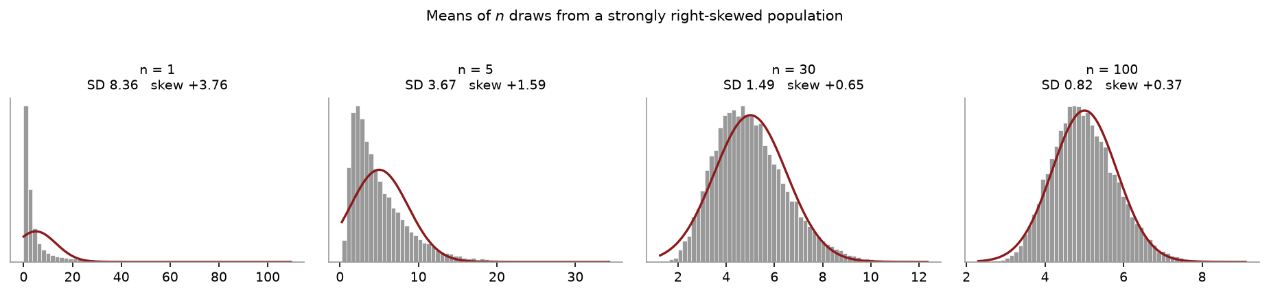
The population on the left is deliberately nasty — strongly right-skewed with a lump near zero, nothing bell-like about it. Read the two numbers in each title as $n$ grows:
| $n$ | SD of $\bar{X}$ | skewness |
|---|---|---|
| 1 | 8.36 | $+3.76$ |
| 5 | 3.67 | $+1.59$ |
| 30 | 1.49 | $+0.65$ |
| 100 | 0.82 | $+0.37$ |
The spread falls like $\sigma/\sqrt{n}$ and the skewness falls like $\text{skew}/\sqrt{n}$, exactly as the chapter claims — and by $n = 100$ the red normal curve sits on the histogram.
Here is the code that drew it. Change the first line and run it again:
N_VALUES = [1, 5, 30, 100]      # <-- change these and re-run
REPS     = 20000                # how many sample means to simulate

import numpy as np
import matplotlib.pyplot as plt
from scipy import stats

rng = np.random.default_rng(250)

def draw(size):
    """A deliberately ugly population: mostly short values, a long right tail."""
    a = rng.exponential(2.0, size)
    b = rng.exponential(12.0, size)
    return np.where(rng.random(size) < 0.30, b, a)

pop = draw(200_000)
mu, sigma = pop.mean(), pop.std()

fig, axes = plt.subplots(1, len(N_VALUES), figsize=(3.1*len(N_VALUES), 2.7))
for ax, n in zip(np.atleast_1d(axes), N_VALUES):
    means = draw(REPS*n).reshape(REPS, n).mean(axis=1)

    ax.hist(means, bins=60, density=True, color="#999999", edgecolor="white")
    xs = np.linspace(means.min(), means.max(), 300)
    ax.plot(xs, stats.norm.pdf(xs, mu, sigma/np.sqrt(n)), color="#8b1a1a", lw=1.6)

    ax.set_title(f"n = {n}\nSD {means.std():.2f}   skew {stats.skew(means):+.2f}")
    ax.set_yticks([])
plt.tight_layout(); plt.show()
Things worth trying.
Set N_VALUES = [1, 2, 3, 4] and watch how slowly it starts — a population this skewed
is nowhere near normal at $n = 4$, which is the honest answer to “is 30 enough?”
Replace draw with rng.normal(100, 15, size). Now even $n = 1$ is a perfect bell,
because the population was already normal and averaging had nothing to fix.
Replace it with rng.uniform(0, 1, size) — flat, not remotely bell-shaped. It converges
in a handful of draws, far faster than the skewed case. How fast the CLT works depends
on how far the population starts from normal, and this is the cheapest way to see it.
Set REPS = 200 instead of 20,000. The bell gets lumpy — a reminder that you are
looking at a simulation, not the theorem itself.
Applying the CLT to one observation. The most common error in this chapter. The theorem is about $\bar{X}$. A skewed population stays skewed no matter how many samples you take from it.
Believing $n = 30$ is a threshold. It is a convention. For a symmetric population $n = 10$ may be ample; for the population in the table above, 30 is roughly the floor, and not enough for a one-tailed statement.
Trusting a two-sided result as evidence the approximation works. The $n = 4$ row shows why: errors in the two tails can cancel and leave the total looking perfect. Check the tails separately.
Thinking the CLT makes the population normal. It does not change the population at all. Standardising does not either — Chapter 3 made that point, and it is the same point. The CLT is a statement about what happens when you average.
Forgetting the standard error. Using $\sigma$ in place of $\sigma/\sqrt{n}$ when standardising $\bar{X}$ produces a $z$ that is $\sqrt{n}$ times too small.
A population has $\mu = 50$, $\sigma = 15$, and is heavily right-skewed. A sample of 100 is drawn. (a) What is the approximate distribution of $\bar{X}$? (b) Find $\mathrm{P}(\bar{X} < 47)$. (c) Find $\mathrm{P}(X < 47)$ for a single observation, or explain why you cannot.
Explain why the normal distribution turns up so often in practice. Your answer should use the word “sum” or “average”.
A binomial has $n = 40$ and $p = 0.08$. Is the normal approximation appropriate? Show the check.
In the skewed-population table, the “inside” share at $n = 4$ is 0.953, almost exactly the nominal 0.95. Explain why this is not evidence that the approximation works at $n = 4$.
A quantity is the sum of 200 small independent effects, none of them normal and none dominant. What can you say about its distribution, and which theorem licenses it?
(a) Approximately $N(50, 15^2/100)$, i.e. mean 50 with standard error $15/\sqrt{100} = 1.5$. (b) $z = (47 - 50)/1.5 = -2.00$, so $\mathrm{P}(\bar{X} < 47) = 0.0228$. (c) You cannot. The population is right-skewed, and the CLT applies only to $\bar{X}$. Without the population’s actual distribution there is no way to get a probability for a single observation.
Because so many measured quantities are themselves sums or averages of many small independent contributions — a person’s height, a firm’s monthly revenue, a measurement error. The CLT says such sums approach normality whatever the individual pieces look like, so the bell appears everywhere without anyone arranging it.
$np = 40(0.08) = 3.2$, which is below 5, so the approximation is not appropriate. ($n(1-p) = 36.8$ passes, but both conditions must hold.) Use the binomial directly.
Because the two tails err in opposite directions and cancel. They are 0.047 and 0.000 against 0.025 each — the left tail is nearly double and the right is empty. The total hides two large, offsetting failures, and any one-tailed statement built on that approximation would be badly wrong.
It will be approximately normal, by the Central Limit Theorem. The conditions that matter are in the question: the effects are independent, there are many of them, and none dominates — so no single component’s shape can impose itself on the total.
Twenty more — the longest set in the book, because this is the result the whole second half rests on and because it is the one people are most confident they have understood. Questions 12, 13 and 19 are the ones that separate reciting the theorem from knowing it.
A population has $\mu = 50$ and $\sigma = 15$ and is heavily right-skewed. A sample of $n = 100$ is drawn. (a) State the approximate distribution of $\bar{X}$, with both parameters. (b) Find $\mathrm{P}(\bar{X} < 47)$. (c) Find $\mathrm{P}(\bar{X} > 52)$. (d) Find $\mathrm{P}(48 < \bar{X} < 53)$.
For the population in question 1, find $\mathrm{P}(X < 47)$ for a single observation, or explain precisely why you cannot.
For each population, state roughly how large $n$ must be before you would trust the normal approximation for $\bar{X}$, and say why. (a) Already normal. (b) Symmetric but with fat tails. (c) Mildly right-skewed. (d) Severely right-skewed, like income. (e) Binary (0/1) with $p = 0.5$. (f) Binary with $p = 0.02$.
Weight lifted per set in a gym is strongly right-skewed with $\mu = 60$ kg and $\sigma = 24$ kg. A trainer records 36 sets. (a) Find the standard error of the mean. (b) Find $\mathrm{P}(\bar{X} > 68)$. (c) The trainer’s own 36 sets averaged 68 kg. Is this good evidence they lift more than the gym average? Give the number that justifies your answer.
State the Central Limit Theorem in your own words. A complete answer says three things: what becomes normal, what its mean and standard deviation are, and what is required of the population.
$X \sim \text{Bin}(100, 0.3)$. (a) Find the mean and standard deviation. (b) Approximate $\mathrm{P}(X \leq 25)$ using the normal with a continuity correction. (c) The exact binomial answer is 0.1631. How close did you get?
Repeat 6(b) without the continuity correction. (a) What answer do you get? (b) By how much does it miss, and in which direction? (c) When does the correction stop mattering?
For each, say whether the normal approximation to the binomial is appropriate, and state the check. (a) $n=50$, $p=0.4$. (b) $n=50$, $p=0.05$. (c) $n=400$, $p=0.01$. (d) $n=25$, $p=0.5$.
Time between arrivals is exponential with a mean of 8 minutes — a distribution nothing like a bell. The mean of 50 such times is recorded. (a) Find the standard error. (b) Find $\mathrm{P}(\bar{X} > 10)$. (c) Which theorem licensed you to use the normal table on an exponential population?
An insurer expects 40 claims next month, each with mean $500 and standard deviation $200, independently. (a) Find the expected total and its standard deviation. (b) Find the probability the total exceeds $22,000. (c) Which quantity did the CLT apply to here — the mean or the sum?
Write down the standardisation for a sum and for a mean side by side. Explain why one has $\sqrt{n}$ multiplying and the other has $\sqrt{n}$ dividing.
For each statement, say whether the CLT supports it. (a) “With a large sample, the population becomes normal.” (b) “With a large sample, the sample data look normal.” (c) “With a large sample, the sample mean is approximately normal.” (d) “With a large sample, individual observations are approximately normal.” (e) “The CLT is why $s$ approaches $\sigma$.”
Name three situations in which the CLT does not rescue you, and say what fails in each.
In a simulation, 1,000 samples of $n = 36$ are drawn from a skewed population and a 95% interval is built each time. 919 of them contain $\mu$. (a) What should the number have been? (b) Is 919 close enough to call the approximation adequate? Justify. (c) At $n = 200$ the figure rises to 939. What does that trend tell you?
The skewness of a sample mean is the population skewness divided by $\sqrt{n}$. (a) A population has skewness 3. Find the skewness of $\bar{X}$ at $n = 9$, $n = 36$ and $n = 144$. (b) Explain how this formula makes the “how large is large enough” question quantitative rather than a matter of folklore.
Explain why so many naturally occurring measurements — heights, measurement errors, test scores — are approximately normal, when nothing arranged for them to be.
A population has $\mu = 100$ and $\sigma = 20$. Compare $\mathrm{P}(X > 110)$ for a single observation, assuming normality, with $\mathrm{P}(\bar{X} > 110)$ for $n = 25$. Explain the gap in one sentence.
“Thirty is large enough” is repeated everywhere. (a) Is it a theorem? (b) Where does the number come from? (c) Give a case where 30 is far too few and one where 5 would do.
Two populations have the same $\mu = 20$ and the same $\sigma = 5$. One is normal and one is a heavily skewed distribution of waiting times. Samples of $n = 100$ are drawn from each. (a) Are the two sampling distributions of $\bar{X}$ the same? (b) Are the two populations’ distributions the same? (c) What does the pair of answers tell you about what a sample mean throws away?
You are designing a study of household electricity use, which you know from previous work is severely right-skewed with a handful of very large users. Your budget allows $n = 40$ or $n = 400$. Argue, using this chapter, for the figure you would choose and say what specifically you are buying.
(a) Approximately $N(50,\ 1.5^2)$: mean 50, standard error $15/\sqrt{100} = 1.5000$. (b) $z = (47-50)/1.5 = -2.00$, so $\mathrm{P} = 0.0228$. (c) $z = (52-50)/1.5 = 1.3333$, so $\mathrm{P} = 0.0912$. (d) $z$ runs from $-1.3333$ to $2.00$, so $\mathrm{P} = 0.9772 - 0.0912 = 0.8860$.
You cannot. The CLT describes $\bar{X}$, not $X$. For a single observation you would need the population’s actual distribution, and all you have been told is that it is right-skewed with a particular mean and standard deviation — which is consistent with infinitely many shapes, giving different answers for $\mathrm{P}(X < 47)$. No sample size changes this: $n$ affects the mean’s distribution, not an individual’s.
(a) Any $n$, including 1 — the mean of normal draws is exactly normal, no approximation involved. (b) Moderate, perhaps 30 to 50: fat tails make extreme draws more common, so more averaging is needed to tame them. (c) Around 20 to 30 is usually ample. (d) Several hundred. Severe skew is slow to average away, and the one-tailed probabilities stay wrong long after the two-tailed ones look fine. (e) About 20 — at $p = 0.5$ the distribution is already symmetric, so only the discreteness needs smoothing. (f) Several hundred: $np \geq 5$ requires $n \geq 250$ on its own.
(a) $24/\sqrt{36} = 4.0000$ kg. (b) $z = (68-60)/4 = 2.00$, so $\mathrm{P} = 0.0228$. (c) It is reasonable evidence. If the trainer were an average lifter, a 36-set mean of 68 kg or more would arise about 2.3% of the time — unlikely enough to doubt the assumption. Note what made this possible: the population of individual sets is badly skewed and we could say nothing about one set, but averaging 36 of them produced a quantity the normal table handles.
The sample mean $\bar{X}$ of $n$ independent draws becomes approximately normally distributed as $n$ grows. Its mean is the population mean $\mu$ and its standard deviation is $\sigma/\sqrt{n}$. What is required of the population is only that it has a finite mean and a finite variance and that the draws are independent — crucially, not that it is normal, or symmetric, or continuous.
(a) $\mu = 100(0.3) = 30.0000$ and $\sigma = \sqrt{100(0.3)(0.7)} = \sqrt{21} = 4.5826$. (b) With the correction, $z = (25.5 - 30)/4.5826 = -0.9820$, so $\mathrm{P} \approx 0.1630$. (c) The exact answer is 0.1631, so the approximation is out by about 0.0001 — accurate to three decimal places.
(a) $z = (25 - 30)/4.5826 = -1.0911$, giving $\mathrm{P} \approx 0.1376$. (b) It misses by about 0.0255, roughly 16% of the true value, and it is too small. The reason is geometric: the binomial puts a bar of probability at 25 and the uncorrected normal cuts straight through the middle of it, discarding half the bar. (c) When $n$ is large enough that a single bar is a negligible share of the distribution. At $n = 100$ it still matters; by $n = 1{,}000$ it is usually below the rounding in your answer. It never hurts to include it.
The check is $np \geq 5$ and $n(1-p) \geq 5$. (a) $20$ and $30$. Yes. (b) $2.5$ and $47.5$. No. (c) $4$ and $396$. No, narrowly. (d) $12.5$ and $12.5$. Yes.
(a) $8/\sqrt{50} = 1.1314$ minutes. (b) $z = (10 - 8)/1.1314 = 1.7678$, so $\mathrm{P} = 0.0386$. (c) The Central Limit Theorem. The exponential is about as un-normal as a distribution gets — right-skewed, bounded below at zero, with its mode at the boundary — and none of that matters, because the theorem makes no assumption about the population’s shape. This is the point of the whole chapter: you may use the normal table on a population you know is not normal, provided you are asking about an average.
(a) $E(S) = 40(500) = $20{,}000$ and $\text{SD}(S) = 200\sqrt{40} = $1{,}264.9111$. (b) $z = (22{,}000 - 20{,}000)/1264.9111 = 1.5811$, so $\mathrm{P} = 0.0569$. (c) The sum. The CLT applies to both, since a sum is just $n$ times the mean — but the parameters differ, and using the mean’s standard error of $200/\sqrt{40} = 31.62$ for a question about the total would be out by a factor of 40.
For a sum, $z = \dfrac{S - n\mu}{\sigma\sqrt{n}}$; for a mean, $z = \dfrac{\bar{X} - \mu}{\sigma/\sqrt{n}}$. Both come from the same fact that variances add, giving $V(S) = n\sigma^2$. The sum keeps all of that accumulated variance, so its standard deviation grows as $\sqrt{n}$. The mean divides the sum by $n$, which divides its variance by $n^2$, leaving $\sigma^2/n$ — so its standard deviation shrinks as $\sqrt{n}$. Adding things up makes them more variable; averaging them makes them less.
(a) No — the population is a fixed set of numbers and nothing about it changes when you sample. (b) No — a histogram of a large sample converges on the population’s shape, skew and all; it does not become a bell. (c) Yes — this is the theorem. (d) No — see question 2. (e) No — that $s \to \sigma$ is the Law of Large Numbers, a different result about consistency rather than about shape. (b) and (c) being different is the distinction this chapter exists to make: the histogram of your data and the histogram of the mean across repeated samples are not the same picture.
(i) The population has no finite variance — Cauchy-type heavy tails. The theorem’s hypothesis fails outright, and the mean of a million draws is no better behaved than one. (ii) The draws are not independent — clustered sampling, time series with autocorrelation, students who studied together. The effective sample size is far below $n$, so the standard error is understated, sometimes badly. (iii) $n$ is too small relative to the skew. The theorem is asymptotic; at $n = 10$ from an income distribution it simply has not arrived yet, and the one-tailed probabilities will be wrong in a predictable direction.
(a) About 950 of 1,000 — a 95% interval should contain $\mu$ 95% of the time. (b) Not really. 919 against an expected 950 is a coverage of 91.9% when 95% was claimed, and the shortfall is about three times what sampling variation in the simulation itself would explain. The intervals are too narrow, and anyone using them believes they are being more careful than they are. (c) That the failure is the approximation, not the method. As $n$ rises the coverage climbs towards its nominal level, exactly as the CLT predicts — the intervals were not wrong in principle, they were being used at an $n$ the approximation had not reached.
(a) Skewness 3 gives $3/\sqrt{9} = 1.0000$ at $n=9$, $3/\sqrt{36} = 0.5000$ at $n=36$, and $3/\sqrt{144} = 0.2500$ at $n=144$. (b) Because it tells you how far along you are. If you regard a skewness below about 0.25 as negligible, then a population with skewness 3 needs $n = 144$ and a population with skewness 6 needs $n = 576$ — numbers you can compute rather than guess. “Thirty is enough” is the answer this formula gives for a population with skewness under about 1.4, which is why the rule works for the mildly skewed data textbooks use and fails for income.
Because such measurements are themselves sums or averages of many small independent contributions. A person’s height is the accumulation of a great many genetic and environmental influences; a measurement error is the accumulation of many small independent errors; a test score is the sum of performance on many items. The CLT says any such accumulation tends to normality regardless of what the individual pieces look like, so the bell curve appears throughout nature without anything in nature having arranged it. It is a theorem about addition, not a law of biology.
For a single observation $z = (110-100)/20 = 0.50$, so $\mathrm{P} = 0.3085$. For the mean of 25, the standard error is 4, so $z = 2.50$ and $\mathrm{P} = 0.0062$. One person being 10 above average is unremarkable; twenty-five people averaging 10 above requires them to be unusual collectively, and that is about fifty times rarer.
(a) No. The CLT is a statement about the limit as $n \to \infty$ and contains no number 30. (b) From practice: for the mildly skewed distributions common in textbook examples, the approximation is adequate around $n = 30$, and the figure got repeated until it sounded like a rule. (c) Far too few: household wealth, insurance claims, or any binary variable with $p = 0.01$ — all need hundreds. Five would do: a population already normal, or very nearly so, where no approximation is needed at all.
(a) Yes, approximately — both are approximately $N(20,\ 0.5^2)$, since the CLT delivers the same answer from the same $\mu$ and $\sigma$ whatever the shape. (At $n = 100$ the skewed one will be very slightly off, by question 15’s formula.) (b) No — one is a bell and one is a long-tailed waiting-time distribution. They are not remotely alike. (c) That a sample mean discards almost everything about the shape of the population. It is sensitive to $\mu$ and $\sigma$ and essentially blind to the rest, which is simultaneously why inference about $\mu$ is so portable across fields and why reporting a mean can be so misleading — two populations that no one would confuse produce the same confidence interval.
Choose 400. Severe right skew with a few very large users is precisely the case in which $n = 40$ is not enough: by question 15’s formula, if the skewness is around 4 then at $n=40$ the sample mean still has skewness $4/\sqrt{40} = 0.6325$, which is enough to make one-tailed probabilities and interval endpoints noticeably wrong. At $n = 400$ that falls to $4/\sqrt{400} = 0.2000$. What you are buying is two separate things: a standard error half the size, and — the point of this chapter — the right to use the normal table at all. The second is the one that would have invalidated the study rather than merely widened it.