The question: you have a sample mean. Somebody asks what $\mu$ is. What do you actually say?
A point estimate is one number. “The mean commute is about 28.4 minutes.” $\bar{x}$ is the point estimator of $\mu$, $s^2$ of $\sigma^2$, $\hat{p}$ of $p$.
An interval estimate is a range with a claim attached. “The mean commute is between 26.4 and 30.4 minutes, and I am 95% confident of that.”
$\bar{X}$ is continuous, so
\[\mathrm{P}(\bar{X} = \mu) = 0\]The probability that your sample mean lands exactly on $\mu$ is zero. The statement “$\mu$ is 28.4” is, strictly, certainly wrong.
That is the pedantic objection. The practical one is worse: a point estimate with no $\pm$ hides the thing the reader most needs, which is how much it would have moved had you drawn a different sample. A study of 10 people and a study of 10,000 can produce the same $\bar{x}$. They do not deserve the same confidence, and only an interval says so.
An estimate without a margin is a number pretending to be a measurement.
Start from Chapter 12. The CLT says
\[Z = \frac{\bar{X} - \mu}{\sigma/\sqrt{n}} \ \dot\sim\ N(0,1)\]and the standard normal puts 95% of its area between $-1.96$ and $+1.96$:
\[\mathrm{P}\!\left(-1.96 < \frac{\bar{X} - \mu}{\sigma/\sqrt{n}} < 1.96\right) = 0.95\]Now just do algebra on the inequality inside. Multiply through by $\sigma/\sqrt{n}$, subtract $\bar{X}$, multiply by $-1$ (which flips both inequalities), and read it backwards:
\[\mathrm{P}\!\left(\bar{X} - 1.96\frac{\sigma}{\sqrt{n}} \;<\; \mu \;<\; \bar{X} + 1.96\frac{\sigma}{\sqrt{n}}\right) = 0.95\]Nothing statistical happened in that step. It is rearrangement. But the rearranged version has $\mu$ in the middle, which is the form we can use.
or in words:
\[\textbf{point estimate} \;\pm\; (\textbf{critical value}) \times (\textbf{standard error})\]That shape never changes. Every interval in the rest of this course is these three pieces; only the pieces get swapped. Learn the shape and the later chapters cost you almost nothing.
The critical values you need:
| confidence | $\alpha$ | $z_{\alpha/2}$ |
|---|---|---|
| 90% | 0.10 | 1.645 |
| 95% | 0.05 | 1.960 |
| 99% | 0.01 | 2.575 |
More confidence means a wider interval. There is no free lunch here: you buy certainty with vagueness. A 100% confidence interval is $(-\infty, \infty)$ and it is perfectly correct and perfectly useless.
This is the sentence students get wrong most often, and it is worth being exact.
The interval is random. $\mu$ is not.
Correct: if you repeated the whole exercise many times — new sample, new interval each time — then 95% of the intervals you constructed would contain $\mu$. This particular one either does or does not, and you will never find out which.
Wrong: “there is a 95% probability that $\mu$ lies between 26.4 and 30.4.” $\mu$ is a fixed number. It is not wandering in and out of your interval. Once the interval is computed, every quantity in that sentence is fixed and no probability remains.
The confidence is a property of the procedure, not of the one interval in front of you. It is a claim about your method’s track record.
This is not pedantry, and you can measure it. Simulate 1,000 samples of $n = 36$ from a normal population and build an interval from each: 955 of the 1,000 contain $\mu$. The procedure promised 95% and delivered 95.5%. The 45 that missed are not errors — they are the price of admission, and they are exactly what the 5% refers to.
Repeat that on a skewed population at the same $n$ and only 919 contain $\mu$. The interval under-covers, because at $n = 36$ a skewed population has not finished converging and the $t$ interval is slightly too narrow. Raise $n$ to 200 and it improves to 939. That is Chapter 12’s “it depends on the shape”, shown in the one place where it costs you something.
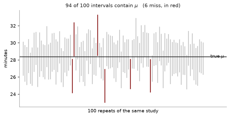
That is the sentence above, drawn. One hundred repeats of the same study, drawn from a population whose $\mu$ we know because we chose it. Each grey bar is one 95% interval; six of them missed, against the five you would expect.
You only ever get one bar. You never learn whether yours is grey or red, and no amount of staring at your own interval will tell you. That is why the 95% belongs to the procedure that generated the bars and not to any one of them.
In the derivation above, $\sigma$ was handed to us. It never is. You have $s$, computed from the same sample, and substituting it costs you something:
\[\bar{x} \;\pm\; t_{\alpha/2,\,n-1}\,\frac{s}{\sqrt{n}}\]The critical value becomes $t$ with $\nu = n - 1$ degrees of freedom — that same $n - 1$ from Chapter 3.
Why? Because $s$ is itself a random variable. With $\sigma$ you have a fixed denominator; with $s$ you have one that jumps around from sample to sample, and when it comes out small the whole ratio blows up. The $t$ distribution’s fatter tails are the distribution being honest about that.
Since $t_{\alpha/2} > z_{\alpha/2}$ always, the $t$ interval is always wider. That extra width is the price of not knowing $\sigma$, and it shrinks fast as $n$ grows:
| $n$ | $t_{0.025,\,n-1}$ | against $z = 1.96$ |
|---|---|---|
| 16 | 2.1314 | 8.7% wider |
| 36 | 2.0301 | 3.6% wider |
| 121 | 1.9799 | 1.0% wider |
A random sample of $n = 36$ staff reports a mean one-way commute of $\bar{x} = 28.4$ minutes.
(a) Suppose past years establish $\sigma = 6$ minutes. Build a 95% interval.
(b) Now suppose $\sigma$ is unknown and this sample gave $s = 6$. Rebuild it.
(c) Which is wider, and why should it be?
The standard error first, since both parts need it:
\[\frac{6}{\sqrt{36}} = \frac{6}{6} = 1 \text{ minute}\](a) With $\sigma$ known, use $z_{0.025} = 1.96$:
\[28.4 \pm 1.96(1) \;\Longrightarrow\; (26.44,\ 30.36)\](b) With $\sigma$ estimated, use $t_{0.025,\,35} = 2.0301$:
\[28.4 \pm 2.0301(1) \;\Longrightarrow\; (26.37,\ 30.43)\](c) The $t$ interval, by about 0.07 of a minute at each end. You estimated $\sigma$ from the same 36 people, so you know less — and the interval is honest about it.
the half-width of the interval. There are exactly three levers.
Raise $n$. The only honest one — but $\sqrt{n}$ means four times the data for half the margin.
Accept less confidence. 90% instead of 95% narrows it immediately. You are simply agreeing to be wrong more often.
Reduce $\sigma$. Not a statistical move. It means measuring more carefully, or studying a more homogeneous population.
Nothing else works. Every “tighter interval” you read about came from one of these three, and it is worth asking which.
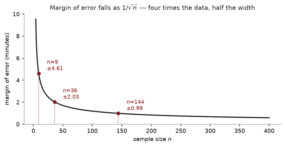
The curve is the first lever drawn. It flattens because $n$ sits under a square root, and the flattening is why survey budgets stop where they do: the first decimal place is cheap and the second costs a hundred times as much.
“Reduce $\sigma$” sounds like advice you cannot act on — $\sigma$ is a fact about the population, not a dial. But look at where it comes from.
Suppose the 36 commuters are really two groups:
| share | mean | SD within the group | |
|---|---|---|---|
| Walkers | 0.40 | 12 min | 3 |
| Drivers | 0.60 | 38 min | 5 |
Nobody in either group varies by much — three minutes and five minutes. Yet the standard deviation of all of them pooled together is $\sigma = 13.4477$. That number did not come from anybody’s commute. It came from the gap between the two groups, and the arithmetic splits cleanly:
\[\underbrace{180.84}_{\text{total}} = \underbrace{0.40(3^2) + 0.60(5^2)}_{\text{within} \;=\; 18.60} + \underbrace{0.40(12-27.6)^2 + 0.60(38-27.6)^2}_{\text{between} \;=\; 162.24}\]Nearly 90% of the variation is the gap between walkers and drivers, not variation in how long anyone’s journey takes. So ask the 36 people which group they are in and sample within each:
| standard error | |
|---|---|
| 36 people, chosen at random | $13.4477/\sqrt{36} = 2.2413$ |
| 36 people, split into the two groups | $\sqrt{18.60/36} = \mathbf{0.7188}$ |
Same 36 people, same budget, one extra question on the form — and a standard error three times smaller. Splitting a sample into groups that are alike on the inside is called stratifying, and it is the cheapest precision in the subject. It is also why a statistician’s first question is about how you are collecting the data, not how much of it you plan to collect.
| Lever | What it costs you |
|---|---|
| Raise $n$ | Money, at four times the rate |
| Lower the confidence level | Meaning — you are claiming less |
| Reduce $\sigma$ | Thought, and sometimes nothing else |
If an exam question asks how to narrow an interval, there are three admissible answers and only one of them is “collect more data”.
Everything so far has produced a two-sided interval, which makes two claims at once. For the commute data, $(26.3699,\ 30.4301)$ says the mean is at least 26.37 and at most 30.43.
Often you only want one of them. If a college is setting a timetable, the question is whether the mean commute is under half an hour; nobody is worried it might be too short. A buyer checking a supplier’s guarantee cares whether the product falls short, never whether it is better than promised.
In that case, stop splitting $\alpha$ between two tails and spend it all on the side you care about:
| tail area used | critical value | upper end | |
|---|---|---|---|
| Two-sided 95% | 2.5% each side | $t_{0.025,35} = 2.0301$ | 30.4301 |
| One-sided 95% | 5% on the right | $t_{0.05,35} = 1.6896$ | 30.0896 |
So we are 95% confident the mean commute is at most 30.0896 minutes — tighter than the two-sided upper end by 0.3405 minutes, from identical data.
What paid for it is the lower end, which is gone. The one-sided interval is
\[(-\infty,\ 30.0896]\]There is no bottom to it. You are not claiming the mean is above anything, and that is exactly the claim you traded away. A two-sided interval spends half its error budget guarding an end you said you did not care about; declining that guard is what buys the tighter top.
The catch. You must choose the direction before seeing the data. Look first, then pick whichever side the data favours, and your stated 5% is really 10% — you gave yourself two chances. Nothing in the finished output reveals that you did it, which is precisely why the discipline matters.
Turn the margin-of-error formula round:
\[n = \left(\frac{z_{\alpha/2}\,\sigma}{E}\right)^{\!2}\]For the commute study, suppose we want the estimate good to $\pm 1$ minute at 95%, with $\sigma \approx 6$:
\[n = \left(\frac{1.96 \times 6}{1}\right)^{\!2} = 138.29 \;\Longrightarrow\; n = 139\]Always round up. 138.29 people cannot be surveyed, and rounding down misses the target.
And note the arithmetic: 36 observations gave us a margin of about 2 minutes. Getting to 1 minute costs 139. That is the $\sqrt{n}$ tax from Chapter 11, in the form you will actually meet it.
The snippets below assume the header and preamble from Chapter 1 — clear all, the log, and a cd to your own folder.
use "DATA/cps_small.dta", clear
ci means wage
    Variable |  Obs   Mean    Std. err.   [95% conf. interval]
        wage | 1,000  10.21302  .1975361   9.825387   10.60065
Read it across: $n$, the point estimate, the standard error ($s/\sqrt{n}$, not $s$), and the interval.
The confidence level is a dial:
ci means wage, level(90)
ci means wage, level(99)
which give widths of 0.650, 0.775 and 1.020 for 90%, 95% and 99% on the same data. Same $\bar{x}$, same standard error — only the critical value moves.
And ci means is not doing anything you cannot do by hand:
quietly summarize wage
display "lower = " r(mean) - invttail(r(N)-1, 0.025)*r(sd)/sqrt(r(N))
display "upper = " r(mean) + invttail(r(N)-1, 0.025)*r(sd)/sqrt(r(N))
These match ci means to the last decimal it prints. There is no magic in the
command — it is the formula above, typed once by StataCorp.
For sample size, there is no special command; it is arithmetic:
display "n = " ceil((invnormal(0.975)*6/1)^2)
import numpy as np
from scipy import stats

xbar, s, n = 28.4, 6, 36
se = s/np.sqrt(n)                       # 1.0
tc = stats.t.ppf(0.975, n-1)            # 2.0301

print(xbar - tc*se, xbar + tc*se)       # 26.3699  30.4301
Or in one call, which also gives it directly from data:
stats.t.interval(0.95, df=n-1, loc=xbar, scale=se) # the same pair
The claim is about the procedure, so test the procedure — build a thousand intervals from a population whose mean you know, and count:
rng = np.random.default_rng(250)
mu, sigma, n, reps = 100, 15, 36, 1000

hits = 0
for _ in range(reps):
    x  = rng.normal(mu, sigma, n)
    lo, hi = stats.t.interval(0.95, n-1, loc=x.mean(),
                              scale=x.std(ddof=1)/np.sqrt(n))
    hits += lo <= mu <= hi

print(hits/reps)        # about 0.95
The ones that miss are not mistakes. They are the 5%, and this is what that number refers to.
Now make the population skewed — swap rng.normal(mu, sigma, n) for
rng.exponential(mu, n) — and re-run. Coverage falls below 0.95, because at $n = 36$ a
skewed population has not finished converging. Raise n and watch it recover.
“There is a 95% probability that $\mu$ is in this interval.” The most-penalised sentence in the course. $\mu$ is fixed; the interval is what was random.
Using $z$ when $\sigma$ was estimated. If you computed $s$ from the data, it is $t$ with $n-1$ degrees of freedom. At large $n$ the difference is cosmetic, but the reasoning is what is being marked.
Using $s$ instead of $s/\sqrt{n}$. The interval comes out $\sqrt{n}$ times too wide, and absurdly so for large samples.
Rounding $n$ down. Round up, always. 138.29 means 139.
Reporting a point estimate alone. Say the margin. If you do not know it, you do not know your estimate.
A sample of $n = 64$ has $\bar{x} = 120$ and $s = 16$. (a) Compute the standard error. (b) Build a 95% confidence interval for $\mu$. (c) Build a 99% interval and state how much wider it is.
A sample of $n = 25$ has $\bar{x} = 48$ and $s = 10$. Build a 95% interval. (Use $t_{0.025,\,24} = 2.0639$.)
Explain the difference between these two sentences, and say which is correct: (a) “95% of the time, $\mu$ falls inside this interval.” (b) “95% of intervals built this way contain $\mu$.”
A researcher wants to estimate a population mean to within 3 units at 95% confidence, believing $\sigma \approx 20$. (a) How many observations are needed? (b) How many to get within 1.5 units? (c) What does the comparison illustrate?
Two studies estimate the same quantity. Study A reports $12.4 \pm 0.3$; Study B reports $12.4 \pm 2.9$. Both used 95% confidence. Give two distinct reasons B’s interval might be so much wider.
(a) $16/\sqrt{64} = 2$. (b) $\nu = 63$, so $t_{0.025} \approx 1.998$: $120 \pm 1.998(2) = (116.00, 124.00)$. (c) $t_{0.005,\,63} \approx 2.656$: $120 \pm 5.31 = (114.69, 125.31)$ — a half-width of 5.31 against 4.00, about 33% wider. Higher confidence, vaguer statement.
$10/\sqrt{25} = 2$, so $48 \pm 2.0639(2) = 48 \pm 4.128 = (43.87,\ 52.13)$.
(b) is correct. Sentence (a) treats $\mu$ as the thing that moves, which it is not — it is a fixed unknown constant. The randomness lives in the sample, hence in the interval. Confidence describes the long-run performance of the procedure.
(a) $n = (1.96 \times 20 / 3)^2 = 170.7$, so 171. (b) $n = (1.96 \times 20 / 1.5)^2 = 683.0$, so 684. (c) Halving the margin roughly quadruples the sample. Precision costs at a rate of $\sqrt{n}$, so each further improvement is more expensive than the last.
Any two of: (i) B had a much smaller sample — the margin goes as $1/\sqrt{n}$, so a margin nearly ten times larger suggests a sample on the order of a hundred times smaller; (ii) B’s population is far more variable, so $\sigma$ or $s$ is larger; (iii) B measured less precisely, inflating $s$ through measurement error. Note that both studies agree on the point estimate — it is the precision, not the finding, that differs.
Fifteen more. The commute data from the worked example runs through the first three, so you can see what changes when only the confidence level moves and nothing else does.
A sample of $n = 36$ commutes gives $\bar{x} = 28.4$ minutes and $s = 6$. (a) Find the estimated standard error. (b) Find the critical value for a 95% interval, stating the degrees of freedom. (c) Build the 95% confidence interval. (d) State the margin of error.
Using the same data, build the 90% and 99% intervals. (a) Give both. (b) Compare the three widths and state the trade-off in one sentence.
Now suppose $\sigma = 6$ were somehow known exactly, with the same $\bar{x}$ and $n$. (a) Build the 95% interval. (b) Compare it with 1(c). Which is wider, by how much, and why?
Explain what “95% confident” means. Then say explicitly what it does not mean.
A 95% interval for a population mean is $(26.37,\ 30.43)$. For each statement, say whether it is true. (a) 95% of the sample values lie between 26.37 and 30.43. (b) There is a 95% probability that $\mu$ lies between 26.37 and 30.43. (c) If the study were repeated many times, 95% of the intervals so constructed would contain $\mu$. (d) A test of $H_0: \mu = 31$ at $\alpha = 0.05$ would reject. (e) A test of $H_0: \mu = 27$ at $\alpha = 0.05$ would reject.
With $\sigma = 6$ and 95% confidence, find the sample size needed for a margin of error of (a) 1.0 minute, (b) 0.5 minutes.
Look at your two answers to question 6. (a) What happened to $n$ when the margin of error halved? (b) Name the three ways to reduce the margin of error, and say which of the three is free.
A 95% confidence interval is reported as $(12.4,\ 19.6)$. Find the point estimate and the margin of error.
A firm claims its mean delivery time is 27 minutes. Using the interval from question 1(c), what do you conclude at the 5% level, and why can you answer without computing a test statistic?
A sample of 16 gives $\bar{x} = 52$ and $s = 8$. (a) Build the 95% interval. (b) Why is the critical value so much larger than 1.96 here?
A student uses $z = 1.96$ for a sample of 16 because “1.96 is the 95% number”. (a) What should they have used? (b) Is their interval too wide or too narrow? (c) What does that do to the interval’s actual coverage?
Two studies estimate the same mean. Study A has $n = 100$, Study B has $n = 400$, and both find $s = 20$. Without computing the intervals, state the ratio of their widths.
A researcher writes: “there is a 95% probability that $\mu$ lies between 26.37 and 30.43.” Rewrite the sentence correctly and explain in one line what is wrong with the original.
Using the data in question 1, construct a one-sided 95% lower bound for the mean commute. Compare the bound with the lower end of the two-sided 95% interval and explain the difference.
The $t$ interval assumes the population is normal. A colleague has $n = 12$ observations from a badly skewed population and builds one anyway. (a) What is the problem? (b) Would $n = 300$ fix it? Which result are you appealing to?
(a) $s/\sqrt{n} = 6/\sqrt{36} = 1.0000$ minute. (b) $\nu = 35$, so $t_{0.025,35} = 2.0301$. (c) $28.4 \pm 2.0301(1.0) = (26.3699,\ 30.4301)$. (d) The margin of error is 2.0301 minutes — the critical value times the standard error, which here happen to be numerically equal because SE $= 1$.
(a) 90%: $t_{0.05,35} = 1.6896$, giving $(26.7104,\ 30.0896)$. 99%: $t_{0.005,35} = 2.7238$, giving $(25.6762,\ 31.1238)$. (b) Widths are 3.3791, 4.0602 and 5.4476 for 90%, 95% and 99%. Higher confidence costs width: you can be more certain of catching $\mu$ only by casting a wider net, and an interval certain to contain $\mu$ would run from minus to plus infinity, which is certain and useless.
(a) With $\sigma$ known the critical value is $z_{0.025} = 1.9600$, giving $28.4 \pm 1.96 = (26.4400,\ 30.3600)$. (b) The $t$ interval from 1(c) is wider, by 0.0702 minutes in each direction. The reason is that $s$ is an estimate with its own sampling variability, and the wider $t$ distribution is the price of not knowing $\sigma$. At $\nu = 35$ that price is small; at $\nu = 8$ it would be substantial.
It means the procedure captures $\mu$ in 95% of repetitions. Build an interval this way from sample after sample, and 95 in 100 of those intervals will contain the true mean. It does not mean there is a 95% probability that $\mu$ lies in the one interval you computed. $\mu$ is a fixed number and your interval is a fixed pair of numbers; either it contains $\mu$ or it does not, and the 95% describes the long-run reliability of the method, not the standing of a particular result.
(a) False — confidence intervals are about the mean, not about where individual observations fall. Most of the data lies well outside this interval. (b) False — see question 4. This is the commonest misstatement in the subject. (c) True. This is the correct reading. (d) True — 31 is outside the interval, and a two-tailed test at $\alpha = 0.05$ rejects exactly the values the 95% interval excludes. (e) False — 27 is inside, so the test does not reject.
The formula is $n = (z\sigma/E)^2$. (a) $n = (1.96 \times 6/1.0)^2 = 11.76^2 = 138.2976$, so round up to $n = 139$. (b) $n = (1.96 \times 6/0.5)^2 = 23.52^2 = 553.1904$, so $n = 554$.
(a) It roughly quadrupled, from 139 to 554. $E$ appears squared in the denominator, so halving it multiplies $n$ by four. (b) Increase $n$; accept lower confidence; reduce $\sigma$. Lowering the confidence level is free in money and expensive in meaning — you get a narrower interval by making a weaker claim, which is not a gain. Reducing $\sigma$ means measuring more precisely or stratifying, which is sometimes possible and is the only genuinely free lunch available. Increasing $n$ costs money, at a quadratic rate.
The point estimate is the midpoint: $(12.4 + 19.6)/2 = 16.0000$. The margin of error is half the width: $(19.6 - 12.4)/2 = 3.6000$. Every reported interval can be read backwards like this, which is worth knowing because papers often print the interval and not the standard error.
27 lies inside $(26.3699,\ 30.4301)$, so you do not reject the firm’s claim at the 5% level. You can answer without a test statistic because the two procedures are algebraically the same thing: a two-tailed test at $\alpha$ rejects $\mu_0$ precisely when $\mu_0$ falls outside the $100(1-\alpha)\%$ interval. The interval is the set of values that would not be rejected.
(a) SE $= 8/\sqrt{16} = 2.0000$ and $t_{0.025,15} = 2.1314$, so the margin of error is 4.2629 and the interval is $(47.7371,\ 56.2629)$. (b) Because $\nu = 15$. With only 16 observations, $s$ is a poor estimate of $\sigma$, and the $t$ distribution compensates by being wider in the tails. The gap from 1.96 to 2.1314 is the cost of that ignorance, and it closes as $n$ grows.
(a) $t_{0.025,15} = 2.1314$. (b) Too narrow — 1.96 is smaller, so the interval is shorter than it should be. (c) Its real coverage is below the advertised 95%: the interval misses $\mu$ more often than once in twenty. The error flatters the result, which is the direction that matters, since it makes the researcher look more precise than the data supports.
Width scales as $1/\sqrt{n}$, so Study B’s interval is $\sqrt{400/100} = 2.0000$ times narrower. Four times the data buys twice the precision, which is the same trade-off as question 7 seen from the other end.
Correctly: “We are 95% confident that $\mu$ lies between 26.37 and 30.43”, or more fully, “this interval was produced by a method that captures $\mu$ 95% of the time.” The original assigns a probability to $\mu$, treating a fixed constant as random; the randomness is in the interval, which varies from sample to sample, not in the parameter, which does not vary at all.
A one-sided 95% lower bound uses $t_{0.05,35} = 1.6896$, putting all 5% in one tail: the bound is $28.4 - 1.6896(1.0) = 26.7104$. It is higher than the two-sided interval’s lower end of 26.3699, and the reason is that the two-sided interval spends half its error allowance guarding the upper end as well. If you genuinely only care about one direction, the one-sided bound is tighter — but you must decide which direction before seeing the data, exactly as with a one-tailed test.
(a) With $n = 12$ there is no normality to appeal to from either direction: the population is not normal, and the CLT has not had enough observations to make $\bar{X}$ normal either. The stated 95% coverage is simply not what the interval delivers, and for a skewed population the two tails will be wrong by different amounts. (b) Yes, broadly — at $n = 300$ the Central Limit Theorem makes $\bar{X}$ approximately normal whatever the population looks like, so the interval recovers close to its nominal coverage. The assumption was never really about the population being normal; it was about $\bar{X}$ being normal, and there are two routes to that.