The question: somebody claims $\mu$ is 25. Is your data consistent with that?
Estimation asked what is $\mu$? and answered with a range. Testing asks something smaller and far more common: a claim arrives from outside the data — a policy document, a contract, a previous study, a competitor’s advertisement — and you have to say whether your sample is compatible with it.
You do not get to answer yes or no. You get to answer surprising or not surprising, and the whole machinery exists to make that word precise.
That is proof by contradiction with a probability attached.
The asymmetry is deliberate. $H_0$ gets the benefit of the doubt in the way a defendant does — and “not guilty” is not the same verdict as “innocent”. Failing to reject is not evidence that $H_0$ is true. It is an absence of evidence that it is false, which is a different and weaker thing.
This is the part Stata cannot do for you, and the part that carries the marks.
| The claim says… | $H_a$ | Tail |
|---|---|---|
| “differs from”, “has changed”, “is there an effect” | $\mu \neq \mu_0$ | two |
| “exceeds”, “is more than”, “has increased” | $\mu > \mu_0$ | right |
| “is less than”, “has fallen”, “fewer” | $\mu < \mu_0$ | left |
| “at least”, “guarantees”, “meets the standard” | $\mu < \mu_0$ | left — you test against the guarantee |
Two questions, in this order. What number is being claimed? That is $\mu_0$. What would I have to show to overturn it? That is $H_a$.
The last row catches people. A guarantee is tested from the side of whoever the guarantee protects: a buyer told “at least 500 hours” looks for evidence that it fails. A target, by contrast, is tested two-tailed, because missing it in either direction is a problem.
Choose the direction before you look at the data. Picking the tail afterwards halves your p-value for free. It has a name — p-hacking — and we will measure what it does later in this chapter.
Both ask: how many standard errors is my sample mean from the value $H_0$ claims?
Same $z$-or-$t$ question as Chapter 13 — is the denominator known, or estimated from the same data? In practice it is nearly always $t$.
The numerator is signal, the denominator is noise. A test statistic is a signal-to-noise ratio and nothing more. Which immediately tells you something uncomfortable: there are two ways to make it large, a bigger gap or a smaller standard error, and only the first is about the effect.
Write all eight down every time until you stop needing to. Exams give marks for the steps, not only the arithmetic.
| Write the decision rule. Critical value and tail: “reject if $ | t | > 2.0301$”. |
Steps 1 to 5 happen before you look at a single number. That ordering is the entire protection against fooling yourself, and a marker can see from the order of your working whether you kept it.
Rejection region. Pick $\alpha$, find the critical value, reject if the statistic lands beyond it. Set up before you see the data.
p-value. Compute the probability of data at least this extreme if $H_0$ were true. Reject if $p < \alpha$.
They always agree. The p-value is the rejection region read backwards — it reports how far past the line you landed, not merely that you did.
The same $n = 36$ staff from Chapter 13: $\bar{x} = 28.4$, $s = 6$. Management’s planning document assumes the mean commute is 25 minutes.
| step | ||
|---|---|---|
| 1 | hypotheses | $H_0: \mu = 25$ against $H_a: \mu \neq 25$ (two-tailed) |
| 2 | test | one mean, $\sigma$ unknown $\Rightarrow$ one-sample $t$, $\nu = 35$ |
| 3 | $\alpha$ | 0.05 |
| 4 | decision rule | reject if $\lvert t\rvert > 2.0301$ |
| 5 | data | $n = 36$, $\bar{x} = 28.4$, $s = 6$ |
| 6 | compute | SE $= 1$, $t = (28.4 - 25)/1 = 3.4$, $p = 0.0017$ |
| 7 | conclusion | $3.4 > 2.0301$ and $p < 0.05$ $\Rightarrow$ reject $H_0$ |
| 8 | meaning | the mean commute is not 25 minutes; it appears about 3.4 minutes longer, so the planning figure is too low |
Why two-tailed? Nothing in the question says management’s figure is too low — only that it is “assumed”. No direction is given, so both must be allowed.
Every test you meet this term fills in that same table. Only rows 2, 4 and 6 ever change.
Your working weight on a gym machine averaged 65 lb. You start a new routine, and over the next block you log 20 sessions: $\bar{x} = 72$ lb, $s = 12$ lb.
(a) You believe the routine made you stronger. State the hypotheses. (b) Test at $\alpha = 0.05$. (c) Redo it two-tailed. (d) What if you had only logged 10 sessions, with the same $\bar{x}$ and $s$?
(a) “Stronger” names a direction, so one tail pointing up: $H_0: \mu = 65$ against $H_a: \mu > 65$.
(b) SE $= 12/\sqrt{20} = 2.6833$, so $t = (72-65)/2.6833 = 2.6087$ with $\nu = 19$. The critical value is $t_{0.05,19} = 1.7291$. Since $2.6087 > 1.7291$, reject. One-tailed $p = 0.0086$.
(c) Two-tailed: critical $\pm 2.0930$, and $p = 0.0173$ — exactly double. Still a rejection, but you spent twice the evidence for it.
(d) With $n = 10$: SE $= 3.7947$, $t = 1.8447$, $\nu = 9$.
| statistic vs critical | verdict | $p$ | |
|---|---|---|---|
| one-tailed | $1.8447 > 1.8331$ | reject | 0.0491 |
| two-tailed | $1.8447 < 2.2622$ | do not reject | 0.0982 |
Same data. Opposite verdicts. Which is why the tail is chosen from your question before you lift, and never from the numbers afterwards.
Here is the definition, and every word is load-bearing:
the probability of getting data at least this extreme, if $H_0$ were true
Say your result out loud as a sentence. For the gym test, $p = 0.0086$:
“If the routine had done nothing at all, I would see a jump this big or bigger about 9 times in 1,000 blocks of training.”
It is an area under a curve, not a verdict a computer reached. For the commute test, $2 \times \mathrm{ttail}(35, 3.4) = 0.0017$ reproduces Stata’s p-value exactly.
This is the fact that changes how you read research.
Draw a fresh sample, test the same true hypothesis, record $p$. Do it a thousand times. If a p-value measured truth, it would come out small every time or large every time. Here is what it actually does — 1,000 tests, $H_0$ true in every one:
| $p < 0.05$ | 50 of 1000 |
| $p < 0.10$ | 105 of 1000 |
| $p < 0.50$ | 479 of 1000 |
| mean $p$ | 0.511 |
The histogram is flat. When $H_0$ is true the p-value is uniform on $[0,1]$: any value is as likely as any other.
Read the first row again. $\alpha$ was 0.05, $H_0$ was true every single time, and we rejected it 50 times out of 1,000. Five per cent. The Type I error rate is not a convention you are asked to trust — it is built into the definition, and that is it measured.
Same test, same $n = 25$. The only change: the true mean is 106, not 100. Now $p$ piles up near zero, and $p < 0.05$ in 476 of 1,000.
That 476 is the power of the test. Sit with it. The effect is genuine, it is six points, it is nearly half a standard deviation — and with 25 observations we miss it more than half the time.
“Not significant” does not mean “no effect”. Here it mostly means $n$ was 25.
Two sentences students write every year, both false.
“$p = 0.03$, so there is a 3% chance $H_0$ is true.” Backwards. $p$ is computed assuming $H_0$ is true — you cannot then use it as the probability of the thing you assumed.
“$p = 0.001$ is a bigger effect than $p = 0.04$.” No. Consider a population whose mean is 100.5 when the claim is 100 — an effect of half a point that nobody would care about:
| $n$ | $p$ | 95% interval |
|---|---|---|
| 25 | 0.927 | — |
| 5,000 | 0.037 | (100.03, 100.87) |
At $n = 5{,}000$ it is “significant”, and the effect is exactly as pointless as before. The interval is what saves you: the whole thing sits within one point of 100. The test says not 100; the interval says not 100, but by at most 0.87.
A big enough $n$ makes any difference significant, because the standard error in the denominator goes to zero. Significance is a statement about $n$ as much as about the effect, which is why a p-value should never be reported on its own.
| $p$ is | $p$ is not |
|---|---|
| the probability of data this extreme, assuming $H_0$ | the probability that $H_0$ is true |
| a measure of how surprising the data is | a measure of how big the effect is |
| small $\Rightarrow$ the data sits badly with $H_0$ | small $\Rightarrow$ the finding matters |
Twenty studies. In every one $H_0$ is true — the true mean is 100 and we test 100. There is nothing to find. Watch anyway:
test 7 gives $p = 0.0159$. Test 20 gives $p = 0.0336$.
Two “significant” findings out of twenty, and not one of them is real. We know that for certain, because the data was generated with no effect in it.
Now imagine running twenty tests and publishing test 7. The arithmetic is correct. The p-value is correctly computed. The finding is nothing at all.
That is what p-hacking is — not fraud, not bad arithmetic, just not telling anyone about the other nineteen. It is also why steps 3 and 4 come before step 5.
| $H_0$ is actually true | $H_0$ is actually false | |
|---|---|---|
| You reject | Type I error, probability $\alpha$ | correct (power, $1-\beta$) |
| You do not reject | correct | Type II error, probability $\beta$ |
Type I — convicting the innocent. You declared an effect that is not there. Type II — acquitting the guilty. There was an effect and you missed it.
You choose $\alpha$. You only influence $\beta$, mostly through $n$. For a fixed $n$, lowering $\alpha$ raises $\beta$ — the only way to cut both is a bigger sample.
$\alpha = 0.05$ is a convention, not a law. Choose it by what the two mistakes cost. A smoke alarm should have a high $\alpha$: false alarms are cheap and misses are not. A murder conviction should not.
The courtroom version above is the standard one. This version is worth having too, because it fixes three things people keep getting wrong.
$H_0$: she is not pregnant — what we assume until the evidence overturns it.
| Not pregnant ($H_0$ true) | Pregnant ($H_0$ false) | |
|---|---|---|
| Test says “pregnant” (reject $H_0$) | Type I — false alarm | correct |
| Test says “not pregnant” (fail to reject) | correct | Type II — a miss |
$H_0$ is the default, not the interesting claim. Nobody sets out to prove somebody is not pregnant. You assume it and ask whether the evidence is strong enough to abandon it.
Failing to reject is not proof. A negative test taken too early does not mean she is not pregnant — it means the evidence is not there yet. This is the cleanest argument for why we say fail to reject rather than accept, and it is the error that costs most marks in this chapter.
The language is already familiar. A test box quoting 99% sensitivity is quoting its power, $1 - \beta = 0.99$. Its false-positive rate is $\alpha$. These are not exam-only quantities; they are printed on the packaging.
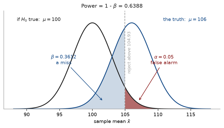
“Lowering $\alpha$ raises $\beta$” is easy to say and easy to forget. Here it is in numbers. A right-tailed test of $H_0: \mu = 100$ with $\sigma = 15$, when the truth is $\mu = 106$:
| $\alpha$ | $n$ | SE | Reject if $\bar{x} >$ | Power | $\beta$ |
|---|---|---|---|---|---|
| 0.05 | 25 | 3.0000 | 104.9346 | 0.6388 | 0.3612 |
| 0.01 | 25 | 3.0000 | 106.9790 | 0.3721 | 0.6279 |
| 0.05 | 100 | 1.5000 | 102.4673 | 0.9907 | 0.0093 |
Rows 1 and 2 are the trade-off: tightening $\alpha$ from 0.05 to 0.01 cut the power from 0.6388 to 0.3721. You made false alarms rarer by making misses far commoner, and a test that misses a real six-unit effect 63% of the time is not a careful test.
Row 3 is the only honest fix. At fixed $n$, $\alpha$ and $\beta$ trade against each other; raising $n$ is the one move that improves both.
The same three numbers, drawn. Two curves — where $\bar{x}$ lands if $H_0$ is true, and where it lands given the truth — and one cut-off between them. The red area is $\alpha$ and the blue area is $\beta$. Slide the dashed line left and the red region grows while the blue shrinks; slide it right and the reverse. You cannot shrink both by moving the line, which is the trade-off made geometric: the only way to shrink both areas at once is to pull the curves apart, and that means a larger $n$.
There is no mathematical reason. The figure comes from Fisher in the 1920s, choosing a round number for a printed table, and it stuck because everybody copied the table.
Other fields chose differently, and were right to. Particle physics demands roughly $\alpha = 0.0000003$ before announcing a discovery. Some medical screening runs at $\alpha = 0.10$ deliberately, because missing a dangerous condition costs far more than calling a patient back for a second test.
So 0.05 is a default, not a fact about the world. Use whatever level the question specifies — and if you are ever asked to justify a level, the answer is always about the relative cost of the two errors, never about statistics.
One data set, two questions:
| 95% CI for mean wage | $(9.8254,\ 10.6007)$ |
| test $\mu = 10.5$ | $p = 0.1466$ — inside, so not rejected |
| test $\mu = 10.7$ | $p = 0.0139$ — outside, so rejected |
A two-tailed test of $\mu = \mu_0$ at level $\alpha$ rejects exactly when the $(1-\alpha)$ confidence interval excludes $\mu_0$.
Not a coincidence — the interval was built from the same inequality the test checks.
Which makes the interval the more useful object: it tests every possible claim at once. Any value inside survives at 5%, any value outside is rejected. So why learn the test at all? Because it hands you the p-value, which says how far past the line you landed. Report both. The interval gives the size, the p-value gives the surprise.
The snippets below assume the header and preamble from Chapter 1 — clear all, the log, and a cd to your own folder.
use "DATA/cps_small.dta", clear
ttest wage == 5
The output carries everything: Mean, Std. err. (the denominator of $t$), t,
Degrees of freedom, and three p-values across the bottom:
Ha: mean < 5          Ha: mean != 5          Ha: mean > 5
Pr(T < t) = 1.0000    Pr(|T| > |t|) = 0.0000  Pr(T > t) = 0.0000
Stata does not know which test you meant, so it prints all three. You choose, from the wording, before looking. The two one-sided values always sum to 1, and the middle is twice the smaller — they are one computation reported three ways.
For problems that give you summary statistics rather than data, the immediate forms take the numbers directly:
ztesti 16 82.5 6 80        // n, mean, sd, claimed value -- sigma known
ttesti 36 28.4 6 25        // same, sigma estimated
And ttail is the function behind the p-value — the mirror image of invt:
display "p = " 2*ttail(35, 3.4)
invt takes an area and returns a cutoff; ttail takes a cutoff and returns
an area. A critical value is the first question, a p-value is the second.
One call does the whole test:
from scipy import stats
import numpy as np

x = np.array([...])                       # your sample
t, p = stats.ttest_1samp(x, 25)           # tests H0: mu = 25
ttest_1samp returns the statistic and the two-tailed p-value. For a one-tailed
test, halve it — but only after checking the sign points the way your $H_a$ does.
From summary statistics rather than data, the p-value is one line:
t, df = 3.4, 35
print(2 * stats.t.sf(abs(t), df))         # 0.0017, the two-tailed p
print(stats.t.sf(abs(t), df))             # 0.0009, the one-tailed p
That is the chapter’s definition executed: the area in the tails beyond your statistic.
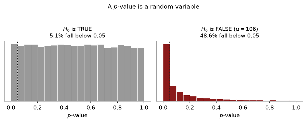
Left: 20,000 tests where $H_0$ is true. The histogram is flat — every p-value is as likely as any other — and 5.1% fall below 0.05. That is $\alpha$, measured.
Right: the same test when $H_0$ is false. Now the p-values pile up near zero, and 48.7% fall below 0.05. That 48.7% is the power: a real six-point effect, missed more than half the time at $n = 25$.
rng = np.random.default_rng(250)
reps, n = 20_000, 25

true  = rng.normal(100, 15, size=(reps, n))    # H0 is TRUE
false = rng.normal(106, 15, size=(reps, n))    # H0 is FALSE

p_true  = stats.ttest_1samp(true,  100, axis=1).pvalue
p_false = stats.ttest_1samp(false, 100, axis=1).pvalue

print((p_true  < 0.05).mean())    # 0.0514  -- the Type I error rate
print((p_false < 0.05).mean())    # 0.4865  -- the power
Change 106 to 103 and the power collapses. Change n to 100 and it recovers.
Power depends on the effect size and the sample size together, and two lines of code
show that faster than any amount of prose.
Putting the equality in $H_a$. It belongs in $H_0$, always.
Choosing the tail after seeing $\bar{x}$. This halves your p-value for nothing and invalidates the test.
“Fail to reject” read as “$H_0$ is true”. You found insufficient evidence. With $n = 25$ you would miss a real six-point effect more than half the time.
Reporting $p$ alone. At a large $n$, significant and trivial are compatible. Give the interval.
Stopping at step 7. A paper that ends at “$p = 0.0017$” has not answered the question. Somebody asked about commutes, not about $t$.
For each, state $H_0$ and $H_a$ and the tail. (a) A bus company advertises a mean journey of 45 minutes; commuters suspect it is longer. (b) Last year’s mean score was 72; the department asks whether this year differs. (c) A supplier guarantees a mean life of at least 500 hours; you are the buyer. (d) A packing machine is set to 500 g; QC checks each morning that it has not drifted.
A sample of $n = 25$ batteries gives $\bar{x} = 486$ hours and $s = 30$. The supplier guarantees at least 500. (a) State the hypotheses and compute $t$. (b) Test at $\alpha = 0.05$, noting that all 5% goes in one tail. (c) The 95% interval is $(473.62,\ 498.38)$. Confirm it agrees.
A study reports $p = 0.04$ from a sample of 50,000. What is the first question you should ask?
Explain why, when $H_0$ is true, p-values are uniformly distributed — and what that implies about running many tests.
A researcher writes: “$p = 0.08$, so we accept the null hypothesis and conclude the treatment has no effect.” Identify two errors.
(a) $H_0: \mu = 45$, $H_a: \mu > 45$, right tail — “suspect it is longer” names a direction. (b) $H_0: \mu = 72$, $H_a: \mu \neq 72$, two-tailed — “differs” is not a direction. (c) $H_0: \mu = 500$, $H_a: \mu < 500$, left tail — the buyer needs evidence the guarantee fails. (d) $H_0: \mu = 500$, $H_a: \mu \neq 500$, two-tailed — drift either way is a fault.
(a) $H_0: \mu = 500$ against $H_a: \mu < 500$. SE $= 30/\sqrt{25} = 6$, so $t = (486-500)/6 = -2.3333$ with $\nu = 24$. (b) One tail, so the critical value is $-t_{0.05,24} = -1.7109$, not $-2.0639$. Since $-2.3333 < -1.7109$, reject. ($p = 0.0142$.) (c) 500 is not in $(473.62,\ 498.38)$, so the interval rejects it too. Agrees.
“What is the confidence interval?” — or equivalently, how big is the effect. With 50,000 observations the standard error is tiny, so a completely trivial difference will clear any significance threshold. The p-value alone cannot distinguish an important finding from a meaningless one.
The p-value is the probability of data at least as extreme as what you saw, computed under $H_0$. If $H_0$ is true, that probability is itself a draw from $[0,1]$ with every value equally likely — $p < 0.05$ happens 5% of the time, $p < 0.10$ happens 10% of the time, and so on. The implication: run enough tests on nothing and some will be “significant” by construction. Twenty tests of true nulls produce about one false positive on average.
(i) You never “accept” $H_0$ — you fail to reject it. (ii) “No effect” does not follow: $p = 0.08$ with a small sample is entirely consistent with a real and substantial effect that the study lacked the power to detect. The honest sentence is “insufficient evidence to reject”, and it should be accompanied by a confidence interval showing what effect sizes remain plausible.
Twenty-five more — the biggest set in the book, because this is the chapter the exam leans on hardest and because almost none of the marks are in the arithmetic. Questions 1 to 4 are set-up only, with no numbers at all; do them first, because a test with the wrong $H_a$ is worth nothing however neatly the rest is computed.
For each, state $H_0$ and $H_a$, and name the tail. (a) A manufacturer claims its cereal boxes average 500 g; an inspector suspects they are underfilled. (b) A training programme is meant to change productivity, and management wants to know whether it has. (c) A supplier guarantees that mean impurity is at most 3 parts per million; you are the buyer. (d) Historically mean class size was 18; the dean asks whether it has changed. (e) A drug company claims a mean recovery time below 7 days; a regulator checks. (f) A machine is calibrated to 250 ml and drifts in either direction. (g) An economist believes a minimum wage rise raised mean hours worked. (h) A bank claims mean wait time is under 4 minutes; a journalist investigates.
In each of these set-ups, something is wrong. Identify it. (a) $H_0: \bar{x} = 50$ against $H_a: \bar{x} \neq 50$. (b) $H_0: \mu > 100$ against $H_a: \mu < 100$. (c) $H_0: \mu = 20$ against $H_a: \mu = 25$. (d) “We will test whether $\mu > 30$, and if the sample mean comes out below 30 we will test whether $\mu < 30$ instead.”
Why does the equals sign always go in $H_0$? Answer by saying what would go wrong in the calculation if it did not.
A researcher collects the data, sees that $\bar{x}$ is above $\mu_0$, and then decides to run a one-tailed test in the upper direction. (a) What is the stated significance level? (b) What is the actual one? (c) Why does this matter more than it sounds like it should?
A machine should fill to 500 g. A sample of $n = 64$ gives $\bar{x} = 497.5$, and $\sigma = 8$ is known from long experience. (a) State the hypotheses. (b) Find the standard error and the test statistic. (c) Find the two-tailed p-value. (d) Conclude at $\alpha = 0.05$ and at $\alpha = 0.01$, and comment on the pair of answers.
A tutoring programme claims to raise scores above the historical mean of 100. A sample of $n = 16$ students gives $\bar{x} = 104$ and $s = 12$. (a) State the hypotheses and the tail. (b) Find the standard error, the test statistic and the degrees of freedom. (c) Compare with the critical value and conclude at $\alpha = 0.05$. (d) Find the p-value.
Repeat question 6 as a two-tailed test. (a) What is the new critical value, and what is the new p-value? (b) The data have not changed. Explain why the conclusion could, in principle, change.
A bottling line is set to 500 ml. A sample of $n = 49$ gives $\bar{x} = 498.2$ and $s = 4.9$. (a) Test at $\alpha = 0.05$, two-tailed, reporting $t$, $\nu$ and the critical value. (b) Find the p-value. (c) State the conclusion in a sentence a plant manager would act on.
For the commute data of Chapter 13 — $n = 36$, $\bar{x} = 28.4$, $s = 6$ — test $H_0: \mu = 30$ against a two-sided alternative at $\alpha = 0.05$. (a) Find $t$ and conclude. (b) The 95% confidence interval is $(26.3699,\ 30.4301)$. Confirm it agrees, and state the general rule.
Using the same commute data, test $H_0: \mu = 31$ instead. (a) Find $t$ and conclude. (b) Does this agree with the interval? Explain how one interval answers infinitely many tests at once.
Which of these is the correct definition of a p-value? For each of the other four, say specifically what is wrong with it. (a) The probability that $H_0$ is true. (b) The probability that $H_0$ is false. (c) The probability of observing data at least as extreme as this, if $H_0$ is true. (d) The probability of making a Type I error. (e) The probability the result is due to chance.
A test returns $p = 0.03$. (a) Conclude at $\alpha = 0.05$. (b) Conclude at $\alpha = 0.01$. (c) Explain why the same data give two different conclusions without either being a mistake.
In a quality-control setting, $H_0$ is “the batch meets specification”. (a) Describe the Type I error in plain words and say who it costs. (b) Describe the Type II error and say who it costs. (c) Which would you rather make if the product is a brake component? A packet of crisps?
$H_0: \mu = 100$ is tested against $H_a: \mu > 100$ at $\alpha = 0.05$ with $n = 25$ and $\sigma = 15$. (a) Find the critical value of $\bar{X}$ — the value above which you reject. (b) Suppose the truth is $\mu = 106$. Find the power of the test. (c) Find $\beta$.
Repeat 14(b) with $n = 100$. (a) What is the power now? (b) State the general relationship between $n$ and power, and why it matters when a study reports “no significant effect”.
Explain the trade-off between $\alpha$ and $\beta$. Why can you not simply set $\alpha = 0.001$ and be safe?
A sample of $n = 5{,}000$ gives $\bar{x} = 100.3$ where $H_0: \mu = 100$, with $\sigma = 5$. (a) Find $z$ and the two-tailed p-value. (b) Now find the same for $n = 25$ with the identical $\bar{x}$. (c) The effect is three-tenths of a unit in both cases. What should be reported alongside the p-value, and why?
A research group runs 20 independent tests at $\alpha = 0.05$, on data where every null hypothesis is in fact true. (a) How many “significant” results do they expect? (b) Find the probability they get at least one. (c) What does this imply about a paper that reports the one significant result out of twenty tests run?
Each of these sentences is wrong. Rewrite it. (a) “We accept the null hypothesis.” (b) “$p = 0.20$, so there is no effect.” (c) “$p = 0.001$, so the effect is large.” (d) “The result is significant, so it is important.” (e) “We reject $H_0$, so $H_a$ is true.”
A test does not reject $H_0$. List three distinct reasons this could happen, only one of which is “$H_0$ is true”.
A test statistic is $z = 1.85$. (a) Find the one-tailed p-value. (b) Find the two-tailed p-value. (c) At $\alpha = 0.05$, which tail choice changes the conclusion?
A student computes $t = -2.45$ with $\nu = 20$ for a left-tailed test, looks up $t_{0.05,20} = 1.7247$, and writes “$-2.45 < 1.7247$, so do not reject.” Identify the error and give the correct conclusion.
List the assumptions behind the one-sample $t$ test, and for each say how you would check it and what you would do if it failed.
Write out the eight steps of a hypothesis test from memory, then use them to test the following: a college claims its graduates earn a mean starting salary of $52,000. A sample of 36 graduates gives $\bar{x} = $49{,}800$ with $s = $7{,}200$. Test at $\alpha = 0.05$ against a two-sided alternative.
Two economists analyse the same dataset. One reports “$p = 0.049$, significant”; the other reports “$p = 0.051$, not significant”. Write a paragraph on what, if anything, separates these two findings.
(a) $H_0: \mu = 500$, $H_a: \mu < 500$ — left. The inspector needs evidence of underfilling. (b) $H_0: \mu = \mu_0$, $H_a: \mu \neq \mu_0$ — two-tailed; “whether it has changed” names no direction. (c) $H_0: \mu = 3$, $H_a: \mu > 3$ — right; the buyer needs evidence the guarantee is breached. (d) $H_0: \mu = 18$, $H_a: \mu \neq 18$ — two-tailed. (e) $H_0: \mu = 7$, $H_a: \mu < 7$ — left; the regulator is checking the company’s claim, and the claim is the thing requiring evidence. (f) $H_0: \mu = 250$, $H_a: \mu \neq 250$ — two-tailed; drift either way is a fault. (g) $H_0: \mu = \mu_0$, $H_a: \mu > \mu_0$ — right. (h) $H_0: \mu = 4$, $H_a: \mu < 4$ — left.
(a) The hypotheses are about $\bar{x}$, a statistic. Hypotheses are always about parameters; you know $\bar{x}$ exactly, so there is nothing to test. (b) $H_0$ has no equals sign, so there is no single value from which to compute a sampling distribution. Write $H_0: \mu = 100$ against $H_a: \mu < 100$. (c) The two hypotheses are not exhaustive — they say nothing about $\mu = 22$. $H_a$ must cover everything $H_0$ does not. (d) The alternative is being chosen after seeing the data, which makes the stated significance level a fiction. See question 4.
Because the whole calculation is conditional on $H_0$ being true, and you cannot compute a sampling distribution from a range of values. “If $\mu = 500$” pins down exactly one distribution for $\bar{X}$, from which a p-value follows; “if $\mu > 500$” pins down none, because the answer would differ for $\mu = 501$ and $\mu = 900$. $H_0$ has to be a specific claim precisely so that it can be contradicted by specific evidence.
(a) Whatever they say — typically 0.05. (b) Effectively 0.10, because they would have run the test in the other direction had the data gone the other way, so there were two chances to reject at 5% each. (c) Because it is invisible in the write-up. The reported test looks like a perfectly ordinary one-tailed test at 5%, and nothing in the published numbers reveals that the direction was chosen after the fact. The discipline of committing to $H_a$ before collecting data is the only thing that makes the stated error rate mean anything.
(a) $H_0: \mu = 500$ against $H_a: \mu \neq 500$. (b) SE $= 8/\sqrt{64} = 1.0000$, so $z = (497.5 - 500)/1.0 = -2.5000$. Note $z$, not $t$ — $\sigma$ is known. (c) $p = 2 \times \mathrm{P}(Z > 2.5) = 2(0.0062) = 0.0124$. (d) At $\alpha = 0.05$: $0.0124 < 0.05$, so reject. At $\alpha = 0.01$: $0.0124 > 0.01$, so do not reject. The data are the same; what changed is how much Type I error you were willing to tolerate. A result sitting between two conventional thresholds is exactly the situation in which reporting the p-value itself, rather than a verdict, earns its keep.
(a) $H_0: \mu = 100$ against $H_a: \mu > 100$ — right tail, because the programme claims to raise scores. (b) SE $= 12/\sqrt{16} = 3.0000$, so $t = (104-100)/3 = 1.3333$ with $\nu = 15$. (c) $t_{0.05,15} = 1.7531$. Since $1.3333 < 1.7531$, do not reject. (d) $p = 0.1012$ — about a one-in-ten chance of a sample mean this high or higher if the programme does nothing.
(a) $t_{0.025,15} = 2.1314$ and $p = 0.2024$, double the one-tailed value. (b) Because the two tests put the 5% allowance in different places. A one-tailed test concentrates all of it in the direction you predicted, making it easier to reject in that direction and impossible to reject in the other. Here the conclusion happens to be the same, but a statistic of, say, 1.80 would have been significant one-tailed and not two-tailed — which is why the tail must be chosen from the question, before the data, and never to secure a result.
(a) SE $= 4.9/\sqrt{49} = 0.7000$, so $t = (498.2 - 500)/0.7 = -2.5714$ with $\nu = 48$. The critical value is $t_{0.025,48} = 2.0106$, and $|-2.5714| > 2.0106$, so reject $H_0$. (b) $p = 0.0133$. (c) “The line is filling below 500 ml. A mean of 498.2 ml across 49 bottles is far enough below target that chance alone would produce it only about 1.3% of the time, so the machine should be recalibrated.” Note that the actionable number is the 1.8 ml shortfall, not the $t$ statistic.
(a) SE $= 6/\sqrt{36} = 1.0000$, so $t = (28.4 - 30)/1.0 = -1.6000$ with $\nu = 35$. The critical value is $t_{0.025,35} = 2.0301$, and $1.6 < 2.0301$, so do not reject. ($p = 0.1186$.) (b) 30 lies inside $(26.3699,\ 30.4301)$, so the interval does not reject it either. The general rule: a two-tailed test of $H_0: \mu = \mu_0$ at level $\alpha$ rejects precisely when $\mu_0$ falls outside the $100(1-\alpha)\%$ confidence interval. They are the same statement rearranged.
(a) $t = (28.4 - 31)/1.0 = -2.6000$, and $2.6 > 2.0301$, so reject. (b) Yes — 31 is outside the interval. The interval is the complete set of null values that would not be rejected at the 5% level, so one interval answers the test for every possible $\mu_0$ at once. This is the strongest practical argument for reporting intervals rather than tests: a test answers one question, an interval answers all of them and shows you the effect size as well.
(c) is correct. (a) and (b) are wrong because the p-value is computed assuming $H_0$ is true — it is a probability about the data, not about the hypothesis. Classical statistics assigns no probability to a hypothesis at all. (d) is wrong because the Type I error rate is $\alpha$, which you choose in advance; the p-value is a property of the data you got. (e) is wrong in a subtler way: “due to chance” sounds like (a) in disguise. The p-value tells you how probable this data is under chance, not how probable chance is given this data — the same inversion as the prosecutor’s fallacy in Chapter 6.
(a) $0.03 < 0.05$, so reject. (b) $0.03 > 0.01$, so do not reject. (c) Because $\alpha$ is not a property of the data — it is a decision about how much Type I error is acceptable, taken before the data arrive and on grounds outside the statistics. At the 1% level you have demanded stronger evidence, and this evidence does not meet that bar while meeting the looser one. Neither verdict is wrong; they are answers to different questions.
(a) Type I: rejecting a batch that was in fact fine. It costs the producer — good output is scrapped or reworked. (b) Type II: passing a batch that was defective. It costs the customer, and ultimately the producer’s reputation. (c) For a brake component, a Type I error is vastly preferable: throw away good parts rather than ship bad ones, so set $\alpha$ high. For crisps, the asymmetry reverses — a slightly underweight packet is a minor matter against the cost of destroying good production, so a lower $\alpha$ is sensible. The choice of $\alpha$ is an economic decision, not a statistical one, and 0.05 is a convention rather than an answer.
(a) SE $= 15/\sqrt{25} = 3.0000$ and $z_{0.05} = 1.6449$, so you reject when $\bar{x} > 100 + 1.6449(3) = 104.9346$. (b) If $\mu = 106$, then $z = (104.9346 - 106)/3 = -0.3551$, so the power is $\mathrm{P}(Z > -0.3551) = 0.6387$. (c) $\beta = 1 - 0.6387 = 0.3613$ — a 36% chance of missing a real six-unit effect.
(a) SE $= 1.5000$, so the cut-off is $100 + 1.6449(1.5) = 102.4673$ and $z = (102.4673 - 106)/1.5 = -2.3551$, giving power $= 0.9907$. (b) Power rises with $n$, because the sampling distributions under $H_0$ and under the truth pull apart as the standard error shrinks. This is why “no significant effect” is uninterpretable without the sample size: at $n = 25$ this test misses a real effect more than a third of the time, so a non-rejection there is weak evidence of anything. The honest report of a null result always includes either the power or, better, the confidence interval showing which effect sizes remain consistent with the data.
For a fixed $n$, shrinking $\alpha$ moves the critical value further out, which makes rejection harder — and that reduces the chance of rejecting a true $H_0$ (good) while also reducing the chance of rejecting a false one (bad). So $\beta$ rises as $\alpha$ falls. You cannot simply set $\alpha = 0.001$ because you would then almost never reject anything, including every genuine effect in the data; a test with a Type I error rate of 0.001 and a Type II error rate of 0.8 is not a careful test, it is a broken one. The only way to reduce both at once is to increase $n$, which is why sample size is the real lever and $\alpha$ is only a dial for choosing which error you fear more.
(a) SE $= 5/\sqrt{5000} = 0.0707$, so $z = 0.3/0.0707 = 4.2426$ and $p < 0.0001$. (b) SE $= 5/\sqrt{25} = 1.0000$, so $z = 0.3000$ and $p = 0.7642$. (c) The confidence interval, or equivalently the effect size with its uncertainty. A difference of 0.3 units may be economically meaningless, and with 5,000 observations the test detects it with overwhelming confidence — the p-value is answering “is the effect exactly zero?”, which is almost never the interesting question. The interval answers “how big is it, and how sure are we?”, which is.
(a) $20 \times 0.05 = 1$. (b) $1 - 0.95^{20} = 1 - 0.3585 = 0.6415$ — about a 64% chance. (c) That the single significant result is roughly what you would expect from nothing at all. A p-value of 0.04 means something when one test was run and very little when it is the best of twenty, because the 5% applies per test and not per paper. The remedies are to report every test run, to adjust the threshold, or to treat the finding as a hypothesis for a fresh dataset rather than as a result.
(a) “We fail to reject the null hypothesis.” You never gather evidence for $H_0$; you only fail to find enough against it. (b) “$p = 0.20$, so there is insufficient evidence of an effect” — ideally with an interval showing what sizes remain plausible. Absence of evidence is not evidence of absence. (c) “$p = 0.001$, so the effect is very unlikely to be zero.” A small p-value reflects the signal relative to the noise, and with a large $n$ a tiny effect produces a tiny p. Size is a separate question, answered by the estimate. (d) “The result is statistically significant.” Importance is a judgement about magnitude and context, which no p-value contains. (e) “We reject $H_0$, so the data are inconsistent with $H_0$ at this level.” Rejection is a decision under an error rate you have chosen to accept, not a proof; one test in twenty rejects a true null by design.
(i) $H_0$ is true, or close enough to true that the data cannot tell. (ii) $n$ is too small — the effect is real but the test lacks the power to detect it, as in question 15. (iii) The data are too noisy, with $s$ inflated by measurement error or an unmodelled source of variation, so a real signal is swamped. A fourth, worth noting: the test was the wrong one — a paired design analysed as independent, for example, which throws away the very structure that would have revealed the effect.
(a) $\mathrm{P}(Z > 1.85) = 0.0322$. (b) $2(0.0322) = 0.0643$. (c) The one-tailed test rejects at 5% ($0.0322 < 0.05$) while the two-tailed test does not ($0.0643 > 0.05$). This is exactly why the tail cannot be chosen after the fact — the same statistic yields opposite verdicts depending on a decision that must be made from the research question alone.
The student has compared a negative statistic with a positive critical value. For a left-tailed test the rejection region is $t < -t_{0.05,20} = -1.7247$, and $-2.45 < -1.7247$, so the correct conclusion is to reject $H_0$. The safe habit is to compare magnitudes — $|{-2.45}| = 2.45 > 1.7247$ — after confirming that the statistic falls on the side $H_a$ predicted. Here it does: a negative $t$ is what a left-tailed alternative expects.
Random sampling / independence. Check it from the study design, not the data — no diagnostic reveals a clustered sample. If it fails, the standard error is wrong, usually too small, and the fix is a method that accounts for the structure. Normality of the population, or a large enough $n$. Check with a histogram or a normal plot of the sample. If it fails and $n$ is small, use a distribution-free test; if $n$ is large, the CLT covers you and nothing needs doing. The data are quantitative and the parameter is a mean. Check that the question is actually about a mean — for counts in categories you want Chapter 17 instead. No outliers driving the result. Check by inspecting the extremes and refitting without them. If a single observation reverses the verdict, say so in the write-up rather than choosing whichever version you prefer.
The steps: (1) state $H_0$ and $H_a$; (2) choose $\alpha$; (3) identify the test statistic and its distribution; (4) state the decision rule; (5) compute the standard error; (6) compute the statistic; (7) find the p-value or compare with the critical value; (8) state the conclusion in the language of the problem. Applying them: (1) $H_0: \mu = 52{,}000$ against $H_a: \mu \neq 52{,}000$. (2) $\alpha = 0.05$. (3) A one-sample $t$, since $\sigma$ is unknown, with $\nu = 35$. (4) Reject if $|t| > t_{0.025,35} = 2.0301$. (5) SE $= 7{,}200/\sqrt{36} = 1{,}200.0000$. (6) $t = (49{,}800 - 52{,}000)/1{,}200 = -1.8333$. (7) $|-1.8333| < 2.0301$, and $p = 0.0753$. (8) Do not reject. There is insufficient evidence at the 5% level that mean starting salary differs from $52,000 — though note the 95% interval, $49{,}800 \pm 2.0301(1200) = (47{,}363.9,\ 52{,}236.1)$, is wide enough to include salaries well below the claim, so this is a statement about the data’s inconclusiveness rather than a vindication of the college.
Essentially nothing separates them. The two p-values differ by 0.002, which is far less than the uncertainty in either, and the only reason they read as opposite findings is that 0.05 happens to sit between them. The threshold is a convention adopted for convenience, not a feature of the world, and nothing changes discretely at 0.05 — the evidence at 0.051 is almost exactly as strong as the evidence at 0.049. The right response is to report both estimates with their confidence intervals, which will be very nearly identical, and to let the reader see that the two studies agree. Treating the pair as a disagreement is an artefact of dichotomising a continuous measure, and it is how a literature ends up with contradictory “findings” drawn from compatible data.