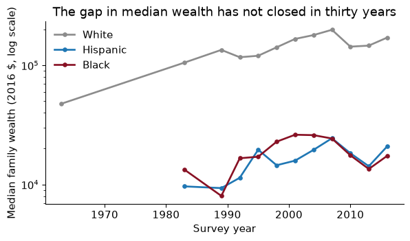
The question: the Federal Reserve’s surveys say the median white family in America holds several times the wealth of the median Black family. Before you repeat a number like that, how do you get from the files someone published to a table you would bet on?
Every empirical paper starts with files, not a regression: a CSV from a statistical agency, a spreadsheet a coauthor emailed, a scraped table. Your first job is to turn them into one table you understand completely. This is wrangling. It takes most of the time in most projects, and it is where most mistakes in applied economics are made, the ones nobody catches, because no referee ever sees your raw files.
Our running example is the racial wealth gap. The Urban Institute has assembled tables from the Survey of Consumer Finances (SCF), the Federal Reserve’s triennial survey of household balance sheets, and from the Census Bureau’s income tables; TidyTuesday republished them in February 2021. In the latest survey year in the file, 2016, the median white family held $171,000 in wealth, the median Black family $17,409 and the median Hispanic family $20,920 (all in 2016 dollars). That is a ratio of 9.8 to 1 between white and Black families. By the end of the chapter we will have checked that number, put it next to homeownership and income, and drawn it.
The single most useful question to ask of any table is: what is one row? A person? A person-year? A county? A county in a year? Hadley Wickham (2014) gave the answer a name. A data set is tidy when
The columns that together pick out exactly one row are the key: (state, year) in a state-by-year panel. If you cannot name the key, you cannot merge, aggregate, or even cluster your standard errors. Tidy is about shape, not cleanliness: a spreadsheet with one column per year is untidy however accurate it is, because “year” is a variable hiding in the column names.
Before you write any code that touches a table, write down in words what one row is and which columns form the key. Then check it.
Checking is one line per table:
tables = {"wealth": (wealth, ["type", "race", "year"]),
          "home":   (home,   ["race", "year"]),
          "income": (income, ["race", "year", "income_bracket"]),
          "debt":   (debt,   ["race", "year"])}
for name, (df, key) in tables.items():
    print(f"{name:7s} {df.shape!s:12s} key unique: {not df.duplicated(key).any()}  "
          f"years {df['year'].min()}-{df['year'].max()}")
wealth  (96, 4)      key unique: True  years 1963-2016
home    (123, 3)     key unique: True  years 1976-2016
income  (2916, 9)    key unique: True  years 1967-2019
debt    (30, 4)      key unique: True  years 1989-2016
All four keys are unique, which is what we hoped. Notice also the year ranges, because they will matter when we merge: the SCF wealth tables are triennial, homeownership is annual, and income starts in 1967.
For each table, say what one row is, in words. (a) wealth. (b) income. (c) Why can you not merge income onto wealth by race and year as it stands?
(a) One row is a statistic (mean or median, the type column) of family wealth for one racial group in one survey year. It is not a family: the microdata are not in the file.
(b) One row is the share of households of one racial group, in one year, whose income falls in one income bracket. There are 9 brackets, so each race-year appears 9 times.
(c) Because the key of income is (race, year, bracket), not (race, year). Merging it by race and year would attach each wealth row to 9 income rows and silently multiply the wealth table’s length. We need to collapse it to one row per race-year first. There is also a smaller problem: income labels groups “White Alone” and “Black Alone”, the wealth table says “White” and “Black”, so the labels must be harmonized too.
Almost everything you do in pandas is one of a handful of verbs (dplyr’s verbs, if you know R):
| Verb | pandas | Does |
|---|---|---|
| select | df[["a", "b"]], .drop(columns=...) |
pick columns |
| filter | df[mask], .query("...") |
pick rows |
| sort | .sort_values(...) |
order rows |
| mutate | .assign(new=...) |
make columns |
| summarize | .groupby(...).agg(...) |
collapse groups to one row |
| group-mutate | .groupby(...).transform(...) |
group statistic on every row |
I write them as a method chain: one verb per line, wrapped in parentheses, read top to bottom like a recipe.
med = (wealth
       .query("type == 'Median' and race in ['White', 'Black', 'Hispanic']")
       .dropna(subset=["wealth_family"])
       .assign(wealth_k=lambda d: d["wealth_family"] / 1_000)
       .sort_values(["race", "year"]))
med.head(3)
The lambda d: inside assign refers to the DataFrame at that point in the chain, which is what lets you use a column you created one line earlier.
groupby is the verb that does the economics. It splits the table into groups, applies a function to each, and combines the answers. agg returns one row per group; transform returns a value for every original row, which is how you demean within a group, compute within-group ranks, or, here, growth since the previous survey:
med = med.assign(
    growth=lambda d: d.groupby("race")["wealth_family"].pct_change(),
    rank_in_year=lambda d: d.groupby("year")["wealth_family"].rank(ascending=False))
loss = (med.query("year in [2007, 2010]")
           .pivot(index="race", columns="year", values="wealth_family")
           .assign(change=lambda d: d[2010] / d[2007] - 1))
Always sort before a within-group pct_change or shift, and always do it inside groupby. Otherwise the first Hispanic year is compared with the last Black year, and pandas will not complain.
Using loss, which group lost the largest share of its median wealth between the 2007 and 2010 surveys?
print(loss["change"].map("{:.0%}".format).to_string())
race
Black       -28%
Hispanic    -25%
White       -28%
Median wealth fell 28% for Black families, 25% for Hispanic families and 28% for white families. In percentage terms the losses were strikingly similar. In dollars they were not: the median white family lost $55,206, the median Black family $6,744. Which is “the” answer depends on the question: relative to where each family stood, the recession hit everyone about equally; as a cushion against the next shock, a 28% loss of a small stock leaves almost nothing. The same groupby gives both. Choosing which to report is economics, not code.
The value in most economic data comes from combining tables: wealth with homeownership, a county file with its covariates, the Opportunity Atlas with a map (Chapter 5). A merge (a join, in database language) matches rows on a key. how= says which unmatched rows to keep:
how= |
Keeps | Stata analogue |
|---|---|---|
"inner" |
keys in both tables | keep(3) |
"left" |
every key in the left table | keep(1 3) |
"outer" |
every key in either | the default |
Merges fail in two ways, and pandas warns you about neither: rows fail to match (a key spelled differently, a missing year), or rows match too many times (a key you thought unique is not, and the table quietly grows). Two arguments make both failures loud:
indicator=True adds a _merge column saying whether each row came from both tables or only one. Look at it every time.validate="one_to_one" (or "many_to_one", "one_to_many") makes pandas check the key’s uniqueness and raise an error if it is wrong.race_map = {"White Alone": "White", "Black Alone": "Black", "Hispanic (Any Race)": "Hispanic"}
inc = (income
.assign(race=lambda d: d["race"].map(race_map))
.dropna(subset=["race"])
[["year", "race", "income_median"]]
.drop_duplicates())
panel = (med[["year", "race", "wealth_family"]]
.merge(home, on=["year", "race"], how="left", validate="one_to_one", indicator="_m_home")
.merge(inc, on=["year", "race"], how="left", validate="one_to_one", indicator="_m_inc"))
print(panel["_m_home"].value_counts().to_dict(), panel["_m_inc"].value_counts().to_dict())
{'both': 33, 'left_only': 1, 'right_only': 0} {'both': 33, 'left_only': 1, 'right_only': 0}
The diagnostics tell a story. One wealth row finds no partner in either table: white wealth in 1963, the only group the 1963 survey tabulated. Homeownership starts in 1976 and the income table in 1967. Neither is a bug; both are facts about the sources you now know. Without the indicator you would have discovered them later, as mysterious missing values.
Now break it on purpose. Merge the uncollapsed income table, whose key is (race, year, bracket):
raw_inc = income.assign(race=lambda d: d["race"].map(race_map)).dropna(subset=["race"])
try:
    med.merge(raw_inc, on=["year", "race"], how="left", validate="one_to_one")
except pd.errors.MergeError as e:
    print("MergeError:", e)
grown = len(med.merge(raw_inc, on=["year", "race"], how="left"))
MergeError: Merge keys are not unique in right dataset; not a one-to-one merge
Duplicates in right:
  year  race
 2019 White
 2019 White
 2019 White
 2019 White
 2019 White ...
With validate= the mistake stops the script. Without it the merge “works” and returns 298 rows from a 34-row wealth table, every wealth number copied once per income bracket, and nothing on the screen looks wrong. A silent many-to-many merge is one of the most common bugs in applied work; validate= costs nine characters.
After a how="left" merge with validate="many_to_one", what must be true about the number of rows? Write the assert.
A left merge keeps every row of the left table, and many_to_one guarantees each left row matches at most one right row. So the result has exactly as many rows as the left table:
out = med.merge(home, on=["year", "race"], how="left", validate="many_to_one")
assert len(out) == len(med), "the merge gained or lost rows"
I put this assertion after every merge I write. It costs nothing and it has saved me more than once.
Tidy data are long, but some calculations are easier wide. The white-to-Black wealth ratio is a comparison across rows of the long table (two races, same year). Pivot so that each race is a column and the ratio is a column operation:
ratio = (med.pivot(index="year", columns="race", values="wealth_family")
            .assign(white_black=lambda d: d["White"] / d["Black"],
                    white_hisp=lambda d: d["White"] / d["Hispanic"]))
ratio[["white_black", "white_hisp"]].round(1).T
pivot goes long to wide; melt goes back. To plot one line per comparison, melt the ratios:
ratios_long = (ratio[["white_black", "white_hisp"]].reset_index()
               .melt(id_vars="year", var_name="comparison", value_name="ratio"))
The log scale makes equal ratios equal vertical distances, which is what you want when the question is “how many times as much”. On a log scale the gap is the vertical distance between the lines, and it has barely moved since 1989.
In which survey year was the white-to-Black ratio of median wealth largest, and what was it?
worst = int(ratio["white_black"].idxmax())
It peaked in 1989, at 16.8 to 1, against 7.9 in 1983 and 7.0 in 1992. Be suspicious of a number that doubles and then halves again. The median Black family’s wealth in 1989, $8,023, is far below the waves on either side, and the SCF samples only a few hundred Black families per wave, so the spike is very likely sampling noise. A ratio of two survey medians has a standard error, which this file does not report. The honest summary is the chart’s: in every other wave since 1983 the ratio lies between 6.2 and 10.8 to one, with no sign of closing.
So far missing values have been an inconvenience to dropna. They deserve much more than that, because how you handle them can change your answer, and the standard defaults change it in predictable directions. This section uses a data set with a lot of real missingness: the Department of Labor’s National Database of Childcare Prices (NDCP), which gives the weekly median price of full-time childcare in every US county from 2008 to 2018, alongside county characteristics from the American Community Survey (TidyTuesday, 9 May 2023).
The economic question is simple. How much does a year of infant care cost, relative to what families earn? The federal guideline is that childcare is “affordable” at 7% of family income. In 2018, 25% of US counties have no infant-care price at all.
Missing data rarely arrive labelled “missing”. In real files you will meet at least five disguises:
NaN in pandas (or None, or pd.NA). The only one pandas understands without being told."NA" (or "N/A", ".", "null"). R writes missing values this way, and TidyTuesday files come from R. The raw childcare file contains the text ,NA 88,636 times. pandas converts "NA" to NaN by default; Polars and DuckDB do not, as we will see."" in a text column, which look like data to every function..mean() will average them happily.survey = pd.DataFrame({"income": [42_000, -2, 55_000, -4, 999_999, 31_000],
"state": ["ME", "NH", "", "VT", "ME", "N/A"]})
print("naive mean:", survey["income"].mean())
clean = survey.assign(
income=lambda d: d["income"].mask((d["income"] < 0) | (d["income"] == 999_999)),
state=lambda d: d["state"].replace({"": np.nan, "N/A": np.nan}))
print("clean mean:", clean["income"].mean(), "| missing:", clean.isna().sum().to_dict())
naive mean: 187998.83333333334
clean mean: 42666.666666666664 | missing: {'income': 3, 'state': 2}
The “naive” mean is nonsense, and it is not obviously nonsense: it is a positive number in the right order of magnitude. The fix is always the same. Read the codebook, find the codes, convert them to NaN with mask or replace, then count.
Counting is not enough; you want to know where the holes are. Three habits:
df.isna().mean() gives the share missing in every column.value_counts(dropna=False) shows NaN as a category, so you see it next to the real values.The childcare data reward the third habit. Missingness falls over time, from 55% of counties in 2008 to 16% in 2016, then rises to 25% in 2018. And in 2018 it is not scattered across the map. It is concentrated in a few states, 10 of which have no county prices at all: CO, DC, FL, GA, IA, IN, LA, MT, NM, NV.
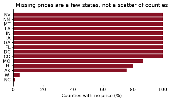
That pattern tells you the mechanism. Prices come from state market-rate surveys, and some states did not report in 2018. A county is missing because of where it is, not because of anything about its own childcare.
Statisticians since Rubin (1976) sort missing data by why the value is missing. The names are terrible; the ideas are simple.
The classic economic case of MNAR is income non-response. In household surveys a large share of people refuse to report their earnings, and refusal is not random: it is more common at the top and the very bottom of the distribution. In the Current Population Survey the Census Bureau imputes earnings for well over a quarter of respondents, and Bollinger and Hirsch (2006) show that because the imputation matches people on observed characteristics only, it biases estimates of things like the union wage premium, whenever the variable you study is not one the imputation matched on. If high earners refuse more, then among people who look alike on paper, the ones who answer are poorer than the ones who don’t, and no amount of conditioning on observables fixes that.
You cannot test MAR against MNAR with the data alone, because the test would need the values you do not have. It is an assumption, and you defend it with knowledge of how the data were collected.
The common responses are:
dropna().To see what each does, we need a case where we know the right answer. So take the 2,360 counties that do have a 2018 price, pretend we have not seen 30% of them, and compare each method’s answer with the truth. I knock out values three ways:
Two quantities to estimate: the average annual price of infant care, and the slope of price on median household income (how many dollars of childcare go with each $1,000 of local income).
The truth, from all 2,360 counties: a mean price of $8,444, a standard deviation of $3,024, and a slope of $147 per $1,000 of income. The estimates:
                             mean price    sd  slope on income
mechanism method
MCAR      listwise                 8477  2964              142
          mean-impute              8477  2492              101
          state-mean-impute        8431  2820              124
MAR       listwise                 8898  3206              150
          mean-impute              8898  2680              112
          state-mean-impute        8599  2952              136
MNAR      listwise                 7724  2548              126
          mean-impute              7724  2136               78
          state-mean-impute        8218  2617              111
Read it a row at a time; each row teaches one thing.
MCAR, listwise. Mean $8,477, slope 142: both close to the truth. When data are missing completely at random, throwing away incomplete rows costs you precision (a smaller sample) but not bias. That is worth remembering, because listwise deletion gets a worse reputation than it deserves.
MCAR, mean-impute. The mean is unchanged, by construction. But the standard deviation falls from $3,024 to $2,492, because 30% of the counties now sit exactly at the mean, and the slope collapses to 101, about 69% of the truth. Mean imputation invents data that have no relationship with anything else, so every relationship is diluted towards zero. Any standard error you compute afterwards is also too small, because the software thinks the invented values are real observations.
MAR, listwise. Now the poorer counties are missing more often, and they have cheaper childcare. The complete-case mean is $8,898, too high. Mean imputation does not help: it fills the holes with that same too-high mean. Filling within state does better, $8,599, because states differ in income and the state mean carries some of the information that predicts missingness. Notice that the slope under listwise deletion is still close to the truth (150). When missingness depends only on a regressor, a regression on complete cases remains unbiased: it is estimating price given income, and conditioning on income is exactly what makes the remaining cases comparable.
MNAR. Expensive counties hide their prices. Every method underestimates the mean (listwise $7,724), and every slope is too flat. Nothing in the data can tell you this has happened. That is why MNAR is the economist’s nightmare: the only defence is knowledge of the process, a validation sample where the values are known, or bounds that ask how wrong you could be (Manski’s partial identification, which you may meet in econometrics).
Listwise deletion is fine under MCAR, and fine for regressions when missingness depends only on the regressors. Mean imputation is almost never what you want for estimation: it keeps the mean and wrecks everything else.
In the table above, price was the outcome of the regression of price on income, and mean-imputing it diluted the slope to 69% of its true value. That is the general rule: do not impute the variable you are trying to explain. Filling missing outcomes with anything predicted from the regressors (a mean, a group mean, a regression prediction) manufactures observations that fit your model by construction, and then you estimate the model on them. Drop rows with a missing outcome, and report how many you dropped and how they differ from the rest.
Imputation is more defensible for features, the right-hand-side variables, especially in prediction. There the missingness indicator earns its keep, because the fact that a value is missing is often information. The Craigslist rent listings of Chapter 9 make the point:
In listings up to 2010, 98% have no square footage, because the site’s format did not ask for it; from 2012 on, 36% still leave it blank. And the blanks are not random. Among listings from 2012 on, the median two-bedroom without a square footage asks $2,219, against $2,442 for one that reports it. Landlords advertise square footage when it is a selling point. A rent model that fills in the median square footage and adds a sqft_missing dummy lets the data tell it that a missing size means a cheaper flat. Without the dummy, the filled-in value would pretend those flats are ordinary.
Chapter 9 made a rule: nothing about the test set may influence how the model is built. Imputation is part of building the model. If you compute the median square footage on the whole data set and then split, the training rows have been filled with a number that used the test rows, and your test score is (slightly) flattering. The fix is the pipeline habit: put the imputer inside the pipeline, so fit learns the median from the training data only and transform applies that same training median to the test data.
from sklearn.model_selection import train_test_split
from sklearn.impute import SimpleImputer
X = recent[["sqft", "beds"]]
X_train, X_test = train_test_split(X, test_size=0.2, random_state=SEED)
leaky = SimpleImputer(strategy="median", add_indicator=True).fit(X)        # wrong: saw the test rows
honest = SimpleImputer(strategy="median", add_indicator=True).fit(X_train) # right
print(leaky.statistics_, honest.statistics_)
[888. 2.] [887. 2.]
add_indicator=True adds the missingness dummies for you. Here the two medians are 888 and 887 square feet, a difference of nothing. The principle matters more than this number. With fancier imputers (filling each hole by a regression or by nearest neighbours) the leaked information is richer, and with small data it can be large.
A hypothetical survey. 1,000 households are asked their income. 800 answer, with a mean of $60,000. The 200 who refuse are, unknown to you, richer, with a true mean of $110,000. (a) What is the true mean income? (b) What do listwise deletion and mean imputation each report? (c) Which mechanism is this, and could imputing by education and age fix it?
(a) $(800 \times 60{,}000 + 200 \times 110{,}000) / 1{,}000 = $70{,}000$.
(b) Listwise deletion reports the mean of the 800 who answered: $60,000. Mean imputation fills the 200 holes with $60,000 and reports $60,000 again, with a standard deviation that is now too small. Both are $10,000 too low; imputation has made the answer look more precise without making it more accurate.
(c) It is MNAR if refusal depends on income itself. Imputing by education and age helps only to the extent that education and age predict both income and refusal; it fixes the part of the problem that is MAR. Whatever is left (the rich refusing more than people with the same education and age) no imputation from observables can touch. That is the Bollinger–Hirsch point about the CPS.
Lecture 05’s checklist is the highest-return habit in this book. Before analysing a new table: read the documentation (universe, units, top-codes, missing codes); look at it (.head(), .sample(10), .info()); summarize (.describe(), .value_counts(dropna=False)); plot the key variables, since a histogram finds a sentinel in seconds; check by group; and check the shape (rows, unique keys, years per unit).
Then turn what you checked into assertions, so the check runs every time the code does. An assert is silent when you are right and stops everything when you are wrong, which is exactly what you want the day a new vintage of the file arrives with a duplicated county.
def check_table(df, key, name=""):
    """Print the facts I want to know about a new table, and fail on a broken key."""
    assert not df.duplicated(key).any(), f"{name}: key {key} is not unique"
    miss = df.isna().mean()
    print(f"{name}: {len(df):,} rows, key {key} unique, "
          f"columns with missing values: {miss[miss > 0].round(2).to_dict()}")

check_table(panel.drop(columns=["_m_home", "_m_inc"]), ["year", "race"], "panel")
shares = income.groupby(["race", "year"])["income_distribution"].sum()
assert shares.between(99.5, 100.5).all(), "bracket shares do not sum to 100"
panel: 34 rows, key ['year', 'race'] unique, columns with missing values: {'home_owner_pct': 0.03, 'income_median': 0.03}
The bracket shares within each race-year should sum to 100. They sum to between 99.8 and 100.2, because each share was rounded to one decimal before publication. So the assertion needs a tolerance, and choosing it forces you to think about why the numbers are not exact.
rent["sqft"].describe() reports a maximum of 900,000 square feet. What do you do?
big = (rent["sqft"] > 10_000).sum()
First, look: 25 listings claim more than 10,000 square feet, a mansion, not a Craigslist flat; almost certainly typos or a lot size in the wrong field. Second, decide in code: rent["sqft"].mask(rent["sqft"] > 10_000) turns them into missing values, which is honest, and keeps their perfectly good rents. Third, write the rule down with the number of rows it affects. Never fix it by deleting rows in Excel: then nobody, including you in six months, can reproduce the table.
Plenty of economic data does not fit comfortably in memory: the CPS since 1962, administrative wage records, a year of taxi trips, scanner data. pandas wants five to ten times a file’s size in RAM, reads every column of a CSV even if you need two, and uses one core. But most “big data” in economics is really medium data: too big for comfortable pandas, easily handled on a laptop with the right file format and engine. You almost never need a cluster.
Our example is two files from the San Francisco housing data (TidyTuesday, 5 July 2022): 200,796 Craigslist rental listings across the Bay Area, 2000–2018, collected by Kate Pennington, and 86,103 building permits filed in San Francisco. Pennington uses them to ask whether new construction raises or lowers nearby rents. They are not large, which is the point: you can see the gains on files small enough to check, and the gains grow with size.
CSV is text, stored row by row. To read one column you parse every byte of every row, and the file stores no types, so the reader must guess whether 02134 is a ZIP code or a number. Parquet stores each column together, compressed and typed, with summary statistics for each chunk, so a reader can fetch only the columns it needs and skip chunks that cannot match a filter.
| Size on disk | pandas read time | |
|---|---|---|
rent.csv |
40 MB | 0.35 s |
rent.parquet |
12 MB | 0.02 s |
rent.parquet, two columns only |
0.001 s |
The Parquet file is 3 times smaller and reads 22 times faster, two columns faster again, and it remembers every column’s type. Anything you will read more than once should be stored as Parquet; converting is one line, pd.read_csv(path).to_parquet(new_path).
Two engines go further. DuckDB is a database that lives inside your Python session: no server, no setup, and it runs SQL directly on files. Polars is a DataFrame library with an expression API much like pandas, and a lazy mode in which you describe the whole query first and the engine works out the cheapest way to run it. Both use every core of your machine and both can process files larger than your memory.
Here is the question from Exercise 06: how many housing units did new-construction permits propose each year, and what did a two-bedroom flat in San Francisco rent for? In DuckDB, one SQL query reads both Parquet files, aggregates each, and joins them, without loading either into pandas:
sf = duckdb.sql(f"""
WITH permits AS (
    SELECT year(CAST(filed_date AS TIMESTAMP)) AS year, sum(proposed_units) AS units
    FROM '{permits_pq}' WHERE permit_type_definition LIKE 'new construction%'
    GROUP BY ALL),
rents AS (
    SELECT year, median(price) AS med_rent, count(*) AS n_listings
    FROM '{rent_pq}' WHERE city = 'san francisco' AND beds = 2
    GROUP BY ALL)
SELECT * FROM rents JOIN permits USING (year) ORDER BY year
""").df()
sf.tail(4)
The answer is a small table you can hand to pandas and matplotlib. Look at n_listings before you look at the rents, though: in 4 of the years the median is based on fewer than 100 listings, so those points are noisy. (And no, this table does not tell you whether construction lowers rents. Booms raise both rents and the incentive to build; the correlation in this table runs the “wrong” way for exactly that reason.)
The same aggregation in Polars, lazily:
q = (pl.scan_parquet(rent_pq)
       .filter((pl.col("city") == "san francisco") & (pl.col("beds") == 2))
       .group_by("year")
       .agg(med_rent=pl.col("price").median(), n=pl.len())
       .sort("year"))
plan = q.explain()
res = q.collect()
Nothing is read when scan_parquet runs. q.explain() prints the plan the optimizer chose, and it shows two tricks: the filter is pushed into the file scan (“predicate pushdown”) and only 4 of the 17 columns are read (“projection pushdown”). .collect() runs it. For the years in both tables, the Polars medians match DuckDB’s exactly; the build checks that with an assert.
One gotcha links this section to the last. Point Polars at the raw CSV and look at the types it chooses:
naive = pl.read_csv(rent_csv)
fixed = pl.read_csv(rent_csv, null_values="NA", infer_schema_length=None)
for col in ["beds", "sqft", "lat"]:
    print(f"{col:5s} naive: {naive.schema[col]!s:7s} with null_values='NA': {fixed.schema[col]}")
beds  naive: String  with null_values='NA': Int64
sqft  naive: String  with null_values='NA': Int64
lat   naive: String  with null_values='NA': Float64
Polars does not treat the string "NA" as missing, so a column of numbers with some "NA"s in it is read as text. No error, no warning; sqft is now a string, and the first time you try to average it you get a confusing failure far from the cause. (DuckDB’s CSV reader does the same.) Telling it null_values="NA" fixes it. The general lesson: every tool has its own default idea of what missing looks like, and you should never rely on a default you have not checked.
A file is too big to load, so you read it in chunks of a million rows with pd.read_csv(..., chunksize=1_000_000). You want the mean rent and the median rent. Which can you compute chunk by chunk?
The mean: keep a running sum and a running count across chunks, and divide at the end. Sums and counts decompose: the total is the sum of the chunk totals. The median does not: the median of the whole file is not the median of the chunk medians, or any other function of them. (Two chunks with medians 1 and 3 can have an overall median anywhere between them, depending on what else is in each.) For medians, quantiles and anything else that needs the whole distribution, use an engine that handles out-of-memory data for you: DuckDB’s median() or Polars’ streaming mode.
Every problem in this chapter (the sentinel, the 900,000-square-foot flat, the states with no prices) is one a picture shows at once. Anscombe (1973) made the point with four tiny data sets that share their means, variances, correlations and regression lines and look nothing alike when plotted. Plot before you trust. Pictures are also how economists communicate: the most-cited results in recent applied micro are figures, like the Opportunity Atlas maps of the next chapter. A good figure is a visual estimator and deserves the same care.
Cleveland and McGill (1984) measured how accurately people read quantities off charts. Position along a common scale is best, then length, then angle and area, with colour last. That ranking explains most of the good advice you will hear:
With tens of thousands of points a scatterplot is an ink blob. The economist’s answer is the binned scatterplot (“binscatter”): cut $x$ into, say, 20 equal-sized bins by quantile, compute the mean of $x$ and of $y$ in each, and plot the 20 points. It is a picture of the conditional mean $E[y \mid x]$, it costs one groupby, and it looks the same whether you have a thousand points or a billion.
def binscatter(df, x, y, bins=20):
    """Means of x and y within quantile bins of x."""
    return (df.assign(bin=pd.qcut(df[x], bins, labels=False, duplicates="drop"))
              .groupby("bin").agg(x=(x, "mean"), y=(y, "mean"), n=(y, "size")))
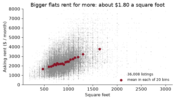
The grey cloud of 36,008 listings says “more space, more rent, lots of noise”, and it is impossible to see where the middle of the cloud is. The garnet bin means show it: rent rises with size roughly in a straight line, with a flat stretch in the middle where large one-bedrooms and small two-bedrooms overlap. A straight line through all the listings has a slope of $1.80 a square foot.
In research you often residualize first, binning the residuals of $x$ and $y$ on controls, so that the slope through the bins is the multiple-regression coefficient (Frisch–Waugh–Lovell). Cattaneo, Crump, Farrell and Feng (2024) show how to choose bins and draw honest confidence bands; their binsreg package does it.
Many groups on one panel, one colour each, is spaghetti. Tufte’s (1983) alternative is small multiples: one small panel per group, on shared axes.
The data are the Luxembourg Income Study’s Gini coefficients, via Our World in Data (TidyTuesday, 5 August 2025), for 45 countries. Each country-year has two Ginis: one for market income, before taxes and transfers, and one for disposable income, after them. The difference is a measure of how much inequality the tax-and-transfer system removes; call it redistribution. In its latest year the United States has a market Gini of 0.51 and a disposable Gini of 0.39, a reduction of 0.112.
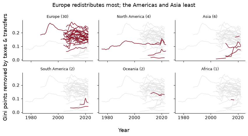
Each panel shows a region’s countries against the grey background of all the others, on shared axes; the background is what makes the comparison (does this region redistribute more than the rest?) possible. The counts in the titles matter just as much. 30 of the 45 countries are European and 1 is African. A claim about “how much countries redistribute” from this sample is a claim about rich democracies.
A classmate plots each country’s latest disposable-income Gini as a bar, in alphabetical order, each bar a different rainbow colour, the y-axis starting at 0.2, titled “GINI DATA”. List what is wrong, and say what you would draw instead to answer “which countries redistribute the most?”
Alphabetical order hides the ranking; the colours encode nothing; the truncated axis makes a bar of 0.30 look twice as long as one of 0.25; the title says nothing; the countries’ “latest years” differ, unannounced. Worst, it plots the wrong quantity: redistribution needs both Ginis.
Draw a dumbbell chart: one row per country, sorted by redistribution, a dot at the market Gini and a dot at the disposable Gini joined by a line. Position on a common scale, both numbers visible, the length of the line is the answer.
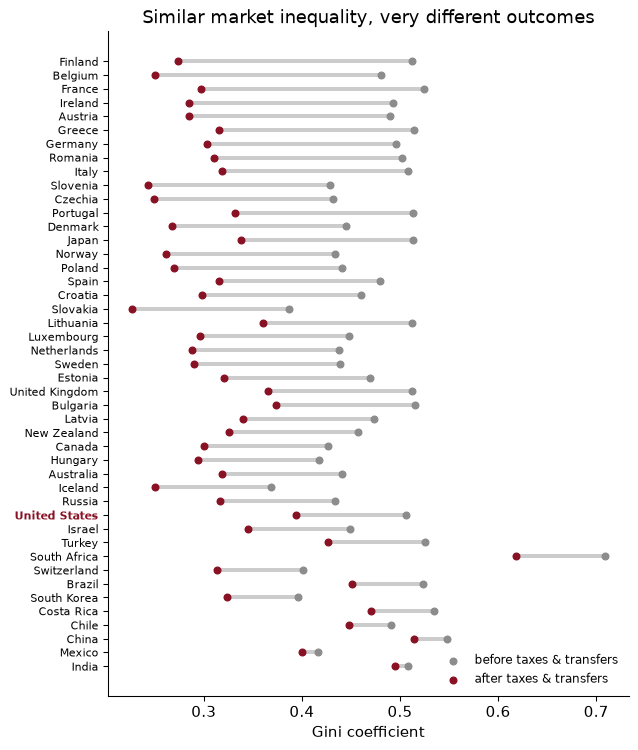
Finland removes the most, 0.238 Gini points; India the least, 0.013. And the chart shows what no bar chart could: market inequality is fairly similar across rich countries, and the big differences in what households live on come from taxes and transfers.
The chapter’s pipeline in one place: load the wealth tables, build a checked race-by-year panel, then the childcare burden with its missing values handled explicitly.
import urllib.request
from pathlib import Path
import numpy as np, pandas as pd
DATA = Path("../data"); DATA.mkdir(exist_ok=True)
TT = "https://raw.githubusercontent.com/rfordatascience/tidytuesday/main/data/"

def fetch(name, url):                                 # download once, then reuse
    path = DATA / name
    if not path.exists():
        urllib.request.urlretrieve(url, path)
    return path

W = TT + "2021/2021-02-09/"
wealth = pd.read_csv(fetch("wealth_race_wealth.csv", W + "race_wealth.csv"))
home = pd.read_csv(fetch("wealth_home_owner.csv", W + "home_owner.csv"))
Median wealth for three groups, merged with homeownership, checked.
med = (wealth.query("type == 'Median' and race in ['White', 'Black', 'Hispanic']")
             .dropna(subset=["wealth_family"])[["year", "race", "wealth_family"]])
panel = med.merge(home, on=["year", "race"], how="left", validate="one_to_one", indicator=True)
assert len(panel) == len(med) and not panel.duplicated(["year", "race"]).any()
wide = panel.pivot(index="year", columns="race", values="wealth_family")
print((wide["White"] / wide["Black"]).round(1).to_dict())
{1963: nan, 1983: 7.9, 1989: 16.8, 1992: 7.0, 1995: 7.0, 1998: 6.2, 2001: 6.4, 2004: 6.9, 2007: 8.2, 2010: 8.2, 2013: 10.8, 2016: 9.8}
The childcare burden in 2018, with missingness counted before anything is dropped.
CC = TT + "2023/2023-05-09/"
cc = pd.read_csv(fetch("tt_childcare_costs_raw.csv", CC + "childcare_costs.csv"))
names = pd.read_csv(fetch("tt_childcare_counties.csv", CC + "counties.csv"))
c18 = (cc.query("study_year == 2018")
         .merge(names, on="county_fips_code", how="left", validate="one_to_one")
         .assign(burden=lambda d: 100 * 52 * d["mc_infant"] / d["mhi_2018"]))
print(f"missing price: {c18['burden'].isna().mean():.1%} of {len(c18):,} counties")
ok = c18.dropna(subset=["burden"])                    # outcome-like: never impute it
w_burden = np.average(ok["burden"], weights=ok["households"])
print(f"household-weighted burden: {w_burden:.1f}% | share of counties above 7%: {(ok['burden'] > 7).mean():.2f}")
missing price: 24.9% of 3,142 counties
household-weighted burden: 19.4% | share of counties above 7%: 1.00
Among counties with a price, a year of infant center care costs on average 19.4% of the county’s median household income (weighting counties by households; 16.3% unweighted), far above the 7% guideline. Only 4 of the 2,360 counties with a price meet the guideline; the cheapest, Mercer County, MO, comes in at 3.3%. (The guideline is about a family’s own income, not the county median, so treat this as a rough comparison.) All of these numbers describe counties in states that reported; whether they describe the rest is an assumption about why the others are missing.
Merging without validate=. A key you believed unique is not, the merge multiplies rows, and every statistic afterwards is quietly reweighted. Merging the wealth table with the uncollapsed income table turned 34 rows into 298 without a word. Nine characters prevent it.
Averaging sentinel codes. −2 for “don’t know”, 99 for “not applicable”, 999,999 for a top-code. They are numbers, so .mean() uses them. Read the codebook and mask them before computing anything.
Mean-imputing and carrying on. It keeps the mean and nothing else: in our experiment it shrank the standard deviation and cut the slope of price on income to 69% of the truth, while making standard errors look smaller. If you impute a feature, add a missingness indicator; never impute the outcome.
Assuming the complete cases are representative. In 2018 the childcare prices are missing for whole states. A national average from the counties that remain is an average for a different country. Tabulate missingness by group before you drop anything, and say what population your answer describes.
Imputing before the split. Fit the imputer on the training data only, inside the pipeline (Chapter 9). Otherwise the test set has helped build the model.
Charts that answer a different question. Alphabetical bars of one Gini, with a truncated axis and rainbow colours, cannot show redistribution. Decide the one comparison the reader should make, then choose the form (dumbbell, small multiples, binscatter) that puts it on a common scale.
For the debt table (student loan debt by race), say in words what one row is, name its key, and check it in code. Which years does it cover, and why can you not merge it with the wealth table for 1983?
Explain, without code, why df.groupby("race")["wealth_family"].pct_change() gives wrong answers if the table is not sorted by year within race. What does the first non-missing growth rate for the second race compare?
Using the 2018 childcare data, compare counties with and without a price on median household income, population and female labour-force participation. Does the comparison support MCAR? Does it tell you anything about MAR versus MNAR?
In the missing-data experiment, the MAR mechanism made the complete-case mean price too high but left the complete-case slope of price on income roughly right. Explain why in two sentences. Would the same be true if missingness depended on price instead of income?
Repeat the missing-data experiment for MCAR with 10%, 30% and 50% of prices removed, and report the mean-imputed slope as a share of the true slope each time. What simple formula does it follow?
Write the Polars equivalent of the DuckDB permits query: new-construction permits per year and units proposed. Check that your numbers match DuckDB’s.
Make a binned scatterplot of the 2018 childcare burden against female labour-force participation (flfpr_20to64) across counties. Then give one causal story in each direction.
Draw a slope chart of redistribution for the countries observed in both 2005 and 2022: two x positions, one line per country, garnet if redistribution rose. In which countries did it rise?
1. One row is the average student loan debt and the share of families with student debt, for one racial group in one survey year; the key is (race, year).
assert not debt.duplicated(["race", "year"]).any()
print(sorted(debt["year"].unique().tolist()), debt["race"].unique().tolist())
[1989, 1992, 1995, 1998, 2001, 2004, 2007, 2010, 2013, 2016] ['White', 'Black', 'Hispanic']
It covers 1989–2016, every SCF wave, for White, Black, Hispanic families. A merge with the 1983 wealth rows would find no debt row: the series starts in 1989. With indicator=True you would see those rows as left_only.
2. pct_change compares each row with the row above it in the table, not with the group’s previous year. Within groupby it restarts at each group, but if the years are out of order it compares, say, 2016 with 1989. Without groupby, the first row of the second race is compared with the last row of the first: a “growth rate” from white wealth in 2016 to Black wealth in 1983, meaningless and indistinguishable from a real one.
3.
cmp = (c18.assign(has_price=c18["mc_infant"].notna())
          .groupby("has_price")[["mhi_2018", "total_pop", "flfpr_20to64"]].median())
print(cmp.round(1).to_string())
           mhi_2018  total_pop  flfpr_20to64
has_price
False       48373.5    21119.0          69.8
True        50341.5    27868.5          70.2
Counties without a price have a median household income of $48,374 against $50,342, and are smaller. So the missing counties are not a random draw: MCAR is out, at least strictly. But since we know prices are missing by state, the differences may be differences between states, which is consistent with MAR given state. The comparison can never distinguish MAR from MNAR, because that would require the missing prices themselves.
4. Under MAR-on-income, the complete cases at each income level are a random sample of the counties at that income level, so the regression of price on income, which only asks about price given income, is unbiased; the mean is biased because the sample has too few low-income (cheap) counties. If missingness depended on price itself, the complete cases at each income level would be the cheaper ones, so the slope would be biased too, as the MNAR rows of the table show.
5.
rng5 = np.random.default_rng(SEED)
for share in [0.1, 0.3, 0.5]:
    obs = full["price"].mask(rng5.random(len(full)) < share)
    filled = full.assign(y=obs.fillna(obs.mean()))
    b = smf.ols("y ~ inc_k", data=filled).fit().params["inc_k"]
    print(f"{share:.0%} missing: slope {b:.0f} = {b / true_slope:.2f} of the truth")
10% missing: slope 133 = 0.91 of the truth
30% missing: slope 105 = 0.71 of the truth
50% missing: slope 73 = 0.50 of the truth
The mean-imputed slope is roughly $(1 - \text{share missing})$ times the true slope: the imputed rows contribute variation in income but none in price, so they pull the covariance down in proportion to their number while leaving the variance of income untouched.
6.
units = (pl.scan_parquet(permits_pq)
           .filter(pl.col("permit_type_definition").str.starts_with("new construction"))
           .with_columns(year=pl.col("filed_date").str.slice(0, 4).cast(pl.Int32))
           .group_by("year").agg(n=pl.len(), units=pl.col("proposed_units").sum())
           .sort("year").collect().to_pandas())
check = units.merge(sf[["year", "units"]], on="year", suffixes=("_pl", "_db"))
print(np.allclose(check["units_pl"], check["units_db"]))
True
The two engines agree year by year. If your version does not, the usual culprit is the date: filed_date is stored as text like 2000-01-03T00:00:00Z, so the year has to be extracted (here, the first four characters) or the text parsed with its time zone. DuckDB’s CAST did that parsing for us silently; Polars insists you say what you mean.
7.
bs7 = binscatter(ok, "flfpr_20to64", "burden", bins=20)
corr7 = ok[["flfpr_20to64", "burden"]].corr().iloc[0, 1]
fig, ax = plt.subplots()
ax.scatter(bs7["x"], bs7["y"], color=GARNET)
ax.set(xlabel="Female labour-force participation, ages 20-64 (%)",
       ylabel="Infant care, % of median income", title="Childcare burden and women's work, 2018")
plt.show()
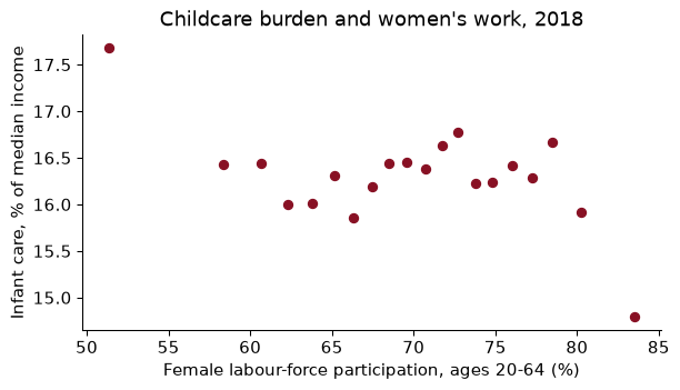
The county-level correlation is -0.08, close to zero. One story: where more mothers work, demand for centre care is higher and prices rise relative to income (participation causes cost). The other: where care is expensive relative to earnings, some mothers stay home (cost causes participation), which would push the relationship negative. The binscatter shows the net of the two, plus everything else that differs between counties. It cannot separate them.
8.
wide8 = gini.pivot(index="Entity", columns="Year", values="redist")[[2005, 2022]].dropna()
rose = wide8[wide8[2022] > wide8[2005]].index.tolist()
fig, ax = plt.subplots(figsize=(5, 4.5))
for c, (a, b) in wide8.iterrows():
    ax.plot([0, 1], [a, b], "o-", color=GARNET if b > a else GREY)
    ax.text(1.03, b, c, va="center", fontsize=8)
ax.set_xticks([0, 1], ["2005", "2022"])
ax.set(ylabel="Gini points removed", title="Redistribution, 2005 vs 2022"); plt.show()
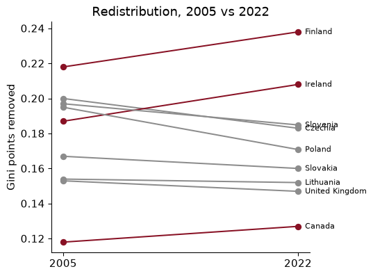
9 countries are observed in both years. Redistribution rose in 3 of them: Canada, Finland, Ireland. With so few countries, and the latest year for each set by survey timing, treat this as description, not a trend in “the world”.
Three papers about what sits behind a published table: who answered, what was filled in for those who did not, and what it takes to stitch sources together.
Meyer, B. D., Mok, W. K. C. & Sullivan, J. X. (2015). “Household Surveys in Crisis.” Journal of Economic Perspectives 29(4): 199–226. doi.org/10.1257/jep.29.4.199
The big federal household surveys are the raw material for most of what we know about income, poverty and transfers, and this paper documents that they are getting worse at their job. Fewer households agree to be interviewed, more of those who do skip individual questions, and the answers they give about programmes like food stamps and welfare fall further and further short of what the administrative records say was paid out. The authors line survey totals up against program totals, which is the “check the data against a number you trust” step of this chapter done at national scale.
Think about: the wealth table in this chapter comes from a voluntary survey. If very wealthy families and very poor families are both less likely to respond, and response differs by race, which way could the published white–Black wealth ratio be pushed, and what outside number would you check it against?
Bollinger, C. R. & Hirsch, B. T. (2006). “Match Bias from Earnings Imputation in the Current Population Survey: The Case of Imperfect Matching.” Journal of Labor Economics 24(3): 483–519. doi.org/10.1086/504276
When someone in the Current Population Survey refuses to report earnings, the Census Bureau fills in the blank with the earnings of a similar-looking respondent. “Similar” means similar on the handful of characteristics the procedure matches on. Bollinger and Hirsch show that if the variable you care about is not one of those, the imputed records carry no information about it, and the gap you estimate (for union members versus non-members, say) is pulled toward zero. Imputation is a modelling choice, and its defaults have consequences for every regression run on the file.
Think about: suppose you filled each missing county childcare price in this chapter with its state’s average, then regressed price on county income within states. Using the match-bias logic, which way would the imputed counties bias the slope, and what would you report alongside it?
Derenoncourt, E., Kim, C. H., Kuhn, M. & Schularick, M. (2024). “Wealth of Two Nations: The U.S. Racial Wealth Gap, 1860–2020.” Quarterly Journal of Economics 139(2): 693–750. doi.org/10.1093/qje/qjad044
The Survey of Consumer Finances only reaches back a few decades, so to see the racial wealth gap over 160 years the authors splice together census returns, state tax records and modern surveys into one series. The gap closed fast in the decades after emancipation and then nearly stopped closing; they argue that differences in what white and Black households own, and the higher capital gains on assets held mostly by white households, help explain the stall. Most of the paper’s work is wrangling: making sources with different units, definitions and coverage mean the same thing.
Think about: some historical sources count wealth per person and modern surveys count it per household. If Black households were on average larger, how would switching from one row definition to the other move the ratio, and why does “what is one row?” become an economic question here?
Reading. Wickham (2014), “Tidy Data”, Journal of Statistical Software. McKinney, Python for Data Analysis, 3rd ed. (2022), chs. 5, 7, 8 and 10, free online, for the pandas verbs, missing data, merges and groupby. Little and Rubin, Statistical Analysis with Missing Data (2019), ch. 1, for the MCAR/MAR/MNAR framework; Bollinger and Hirsch (2006), “Match Bias from Earnings Imputation in the Current Population Survey”, Journal of Labor Economics, for what imputation does to economic estimates. Schwabish (2014), “An Economist’s Guide to Visualizing Data”, Journal of Economic Perspectives; Healy, Data Visualization (2018, free at socviz.co); Cattaneo, Crump, Farrell and Feng (2024), “On Binscatter”, American Economic Review.