The question: official price statistics arrive once a month, weeks after the fact, and many economic quantities are never published as a file at all. How does an economist collect data that live on web servers and web pages, reliably, and within the rules?
In 2007 the government of Argentina began publishing inflation figures that few people believed. Alberto Cavallo, then a PhD student, wrote programs that visited the websites of large Argentine supermarkets every day and recorded the price of every product. His online price index rose more than twice as fast as the official one. That work grew into the Billion Prices Project with Roberto Rigobon at MIT, which collected daily prices from hundreds of retailers in dozens of countries, and into a company whose indices central banks now watch. The obvious objection, that online prices are not the prices people pay, Cavallo (2017) answered with more data: at large retailers that sell both online and in stores, the online and in-store price of the same product were identical about 72% of the time.
That is the pattern of a lot of modern empirical economics. Find a website that records economic behaviour nobody has organized into a data set: prices, job postings, rental listings, newspaper text. Collect it carefully. Validate it against official data. Hershbein and Kahn (2018) used millions of online job postings to show that the Great Recession accelerated employers’ demands for skills. Baker, Bloom and Davis (2016) counted newspaper articles to build an index of economic policy uncertainty. The Craigslist rents of Chapters 4, 5 and 9 were scraped by Kate Pennington.
There are three ways to get data off the web, and you should try them in this order:
This chapter does the second and third. Everything here is a live request to a real server, so every response is saved to ../data/web/ the first time and read from disk afterwards; I explain why in the section on being a good citizen.
The web is a conversation between a client (your Python session, or a browser) and a server. The client sends a request: a method (GET to read, POST to send a body), a URL, and some headers. The server sends back a response: a three-digit status code, its own headers (including the type of content), and a body, which may be HTML, JSON, CSV or anything else.
A URL for an API has three parts:
https://api.worldbank.org/v2/country/USA/indicator/SP.DYN.LE00.IN?format=json&date=2019
└────────── base ────────┘└───────────── endpoint (path) ─────────┘└─── query string ──┘
The query string, after the ?, is a list of key=value parameters joined by &. In Python you never build it by hand; you pass a dictionary to requests and it encodes the parameters for you.
The status code is the first thing to read:
| Code | Meaning | What to do |
|---|---|---|
| 200 | OK | parse the body (and still check it) |
| 301, 302 | redirect | requests follows it for you |
| 400 | bad request | check your parameters |
| 401, 403 | not authorized, forbidden | a missing or wrong API key, or you are blocked |
| 404 | not found | a typo in the address |
| 429 | too many requests | slow down; respect the Retry-After header |
| 500, 503 | server error | not your fault; retry later, with a pause |
Here are three real requests:
probes = {"books catalogue":      "https://books.toscrape.com/",
          "a page that is not there": "https://books.toscrape.com/catalogue/page-999.html",
          "a made-up World Bank indicator": "https://api.worldbank.org/v2/country/USA/indicator/NOT.REAL"}
for label, url in probes.items():
    r = cached_get(url, params={"format": "json"} if "worldbank" in url else None, keep_errors=True)
    print(f"{label:32s} {r['status']}  {r['type'][:24]:24s} {r['text'][:60].strip()!r}")
books catalogue                  200  text/html                '<!DOCTYPE html>\n<!--[if lt IE 7]>      <html lang="en-us" cl'
a page that is not there         404  text/html                '<html>\r\n<head><title>404 Not Found</title></head>\r\n<body>\r\n<'
a made-up World Bank indicator   200  application/json;charset '[{"message":[{"id":"120","key":"Invalid value","value":"The'
The first two are what you expect. The third is the lesson: the World Bank answers a request for an indicator that does not exist with status 200, “OK”, and a body that is an error message. A 200 means the server answered, not that you got data. Always look at what came back.
You run a script that downloads twenty World Bank indicators overnight. In the morning, three of the twenty DataFrames are empty and nothing crashed. Give two possible causes and say how you would make the script fail loudly instead.
First, a mistyped or retired indicator code: the server returns 200 with a message instead of data, as above, and an empty DataFrame follows. Second, a temporary outage that returned an error status your code never checked. (On the day I wrote this chapter, the World Bank’s data endpoints returned 400 for well over an hour for every economic indicator, then recovered.) To fail loudly: call r.raise_for_status(), which raises an exception on any 4xx or 5xx code; then check the content, with an assert that the parsed result has rows and that the expected keys are present. A script that downloads data should be pessimistic: every step checks that it got what it asked for.
Most APIs answer in JSON (JavaScript Object Notation), which is nested dictionaries {} and lists [] of strings, numbers, true/false and null. It maps directly onto Python dictionaries and lists. Here is one record from the World Bank:
r = cached_get("https://api.worldbank.org/v2/country/USA/indicator/SP.DYN.LE00.IN",
               params={"format": "json", "date": "2019"})
meta, records = json.loads(r["text"])
print(meta)
print(records[0])
{'page': 1, 'pages': 1, 'per_page': 50, 'total': 1, 'sourceid': '2', 'lastupdated': '2026-10-08'}
{'indicator': {'id': 'SP.DYN.LE00.IN', 'value': 'Life expectancy at birth, total (years)'}, 'country': {'id': 'US', 'value': 'United States'}, 'countryiso3code': 'USA', 'date': '2019', 'value': 78.7878048780488, 'unit': '', 'obs_status': '', 'decimal': 0}
The response is a list of two things: metadata (how many pages, how many records) and a list of records. Each record is nested: country is itself a dictionary with an id and a value. pd.json_normalize flattens nested records into columns, naming them with dots:
pd.json_normalize(records)[["country.value", "countryiso3code", "date", "value"]]
Without json_normalize, how would you extract the country name and the value from records? Why is the library function better?
A list comprehension that walks the nesting: [{"country": x["country"]["value"], "value": x["value"]} for x in records], then pd.DataFrame(...). It works, but it breaks with a KeyError the first time a record lacks a field, and you must write a new one for every API. json_normalize handles missing fields (they become NaN), flattens any depth, and with record_path= and meta= it can pull a list out of a deeper level while repeating fields from the level above. Write the comprehension once to understand what is happening, then use the library.
The World Bank’s API serves the World Development Indicators, well over a thousand series on everything from GDP to school enrolment, for every country and decades of years, and it needs no key. An indicator has a code: NY.GDP.PCAP.KD is GDP per capita in constant 2015 dollars, SP.DYN.LE00.IN is life expectancy at birth.
APIs rarely send everything at once. They split a long answer into pages and tell you in the metadata how many there are; you ask for page 1, then page 2, until you have them all. That is pagination. Asking for GDP per capita in 2019 for “all” countries, 100 records a page, the metadata says there are 3 pages and 266 records. A loop collects them:
def wb_get(indicator, countries="all", per_page=100, **params):
    """Download every page of a World Bank indicator into a DataFrame."""
    url = f"https://api.worldbank.org/v2/country/{countries}/indicator/{indicator}"
    rows, page = [], 1
    while True:
        r = cached_get(url, params={"format": "json", "per_page": per_page, "page": page, **params})
        meta, data = json.loads(r["text"])
        rows += data or []                    # a page can be empty: `None`
        if page >= meta["pages"]:
            return pd.json_normalize(rows), meta
        page += 1
        time.sleep(0.2)                       # be polite between pages
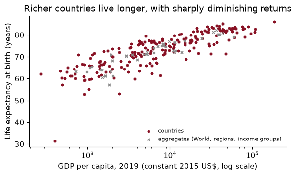
Now three calls and a merge give a cross-country panel, and with it one of the most famous pictures in development economics, the Preston curve (Preston 1975): life expectancy against income per head.
Across 208 countries, each doubling of income per head goes with about 3.2 more years of life expectancy (the slope of life expectancy on log income, times log 2). The curve is concave in levels, which is why the x-axis is on a log scale: an extra $1,000 matters enormously in a poor country and barely at all in a rich one. Preston’s own point was that the curve shifts up over time, so that a country at a given income lives longer today than it would have decades ago, which says that health depends on more than income.
Notice the grey crosses. The “all countries” endpoint also returns 48 aggregates: “World”, “Euro area”, “Low income”, “Sub-Saharan Africa”. If you regress on them along with the countries you have counted China, East Asia and the world all as separate observations. The API’s /country endpoint labels each code with its region, and aggregates have the region “Aggregates”; we keep only real countries.
You want every country’s GDP per capita for every year from 1960 to 2023 (64 years, about 266 country codes including aggregates). How many requests does that take at 100 records per page? At 1,000? Why does the difference matter?
There are about $266 \times 64 \approx 17{,}000$ records. At 100 per page that is about 170 requests; at 1,000 per page, about 17. Fewer, larger requests are faster (each request has a fixed cost of a round trip to the server), kinder to the server, and less likely to run into a rate limit, the cap most APIs put on requests per second or per day. Ask for as much as the API allows per call.
The Federal Reserve Bank of St. Louis’s FRED database has more than 800,000 US and international time series. For quick work it offers any series as a CSV at a stable address, no key needed:
r = cached_get("https://fred.stlouisfed.org/graph/fredgraph.csv", params={"id": "UNRATE,CPIAUCSL"})
fred = pd.read_csv(io.StringIO(r["text"]), parse_dates=["observation_date"], index_col="observation_date")
fred["inflation"] = 100 * fred["CPIAUCSL"].pct_change(12)
fred = fred.loc["1960":].dropna()
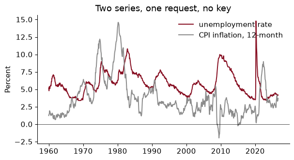
The file runs through September 2026, when unemployment was 4.2% and inflation over the previous twelve months 3.7%. (This copy was downloaded on 2026-10-23; FRED updates as new data are released, which is exactly why you record the date.)
The CSV route gives you the latest numbers. The full FRED API gives you much more: search, metadata, release calendars, and vintages, the data as they were first published before revisions. If you are evaluating a forecast made in 2008, you need GDP as forecasters saw it in 2008, not as it has since been revised. The API needs a free key, and so do the Census, BLS and BEA APIs.
An API key identifies you to the provider so it can enforce limits and, for paid services, bill you. Treat it as a password: anyone who has it can use your quota or run up your bill. Programs scan public GitHub repositories for leaked keys, and find them within minutes.
A key never goes in your code, your notebook or your repository. It goes in an environment variable, set outside the code, which your code reads:
import os
key = os.environ.get("FRED_API_KEY")          # None if it is not set
r = session.get("https://api.stlouisfed.org/fred/series/observations",
                params={"series_id": "GDPC1", "api_key": key, "file_type": "json",
                        "observation_start": "2000-01-01"}, timeout=30)
obs = pd.DataFrame(r.json()["observations"])
obs["value"] = pd.to_numeric(obs["value"], errors="coerce")   # FRED writes missing as "."
(That block is shown but not run when the book is built, because it needs my key.) You set the variable in the terminal, export FRED_API_KEY="...", or, more conveniently, in a file called .env in the project folder, which the python-dotenv package reads with load_dotenv(). The .env file goes in .gitignore before you create it, and you commit a .env.example with fake values so that a collaborator knows which keys to get. Notice the last line, too: FRED’s API marks a missing observation with the string ".", another disguise for missingness from Chapter 4.
You notice that last week you committed a notebook containing your Census API key, and pushed it to GitHub. You delete the cell and push again. Are you safe?
No. Git keeps history: the key is still in last week’s commit, visible to anyone who looks (Chapter 3). And bots may have copied it within minutes of the push. The only fix is to revoke the key on the provider’s website and generate a new one, then put the new one in .env. Rewriting the repository’s history is a good second step, but it cannot un-leak a key that has already been copied. Revoke first.
A server is someone else’s computer. Three habits keep you welcome on it and keep your project reproducible.
Rate limits. Most APIs cap requests: FRED’s API allows 120 a minute; the Census API allows 500 a day without a key. Exceed the limit and you get a 429, or a silent block. Sleep between requests (time.sleep(0.2) in wb_get), and ask for more per request.
Retries with backoff. Servers fail temporarily. Rather than crash, retry, waiting longer each time: 1 second, then 2, then 4. This is exponential backoff, and requests can do it for you when you mount a retry policy on a session:
session = requests.Session()
session.headers.update({"User-Agent": "ECON368-course-book (educational use)"})
session.mount("https://", HTTPAdapter(max_retries=Retry(
    total=4, backoff_factor=1, status_forcelist=[429, 500, 502, 503, 504])))
The session also sends a User-Agent header saying who you are. Some servers require one (Wikipedia and the SEC’s EDGAR do), and it is simply polite.
Caching. Never download the same thing twice. Every request in this chapter has gone through this function, defined when the chapter starts:
def cached_get(url, params=None, keep_errors=False):
    """GET url once and save status, date and body in ../data/web; reuse the file afterwards."""
    key = hashlib.md5((url + json.dumps(params, sort_keys=True)).encode()).hexdigest()[:16]
    f = CACHE / f"{key}.json"
    if f.exists():
        return json.loads(f.read_text())
    r = session.get(url, params=params, timeout=30)
    if "charset" not in r.headers.get("Content-Type", ""):
        r.encoding = "utf-8"                     # e.g. so that "£" decodes correctly
    out = {"url": r.url, "status": r.status_code, "type": r.headers.get("Content-Type", ""),
           "fetched": str(dt.date.today()), "text": r.text}
    if r.ok or keep_errors:                      # never cache a failure by accident
        f.write_text(json.dumps(out))
    time.sleep(0.5)                              # a pause after every real request
    return out
It turns the URL and parameters into a file name, and if that file exists it returns the saved response without touching the network. After a real request it pauses half a second, so that a loop over fifty pages does not hammer the server. It records the date of download, because a web source is not a fixed object: the same request next month can return different numbers. And it refuses to save a failure, so that an outage does not get frozen into your data. After building this chapter once, the cache holds 83 responses, and rebuilding makes no requests at all. That is the reproducibility rule of Chapter 3 applied to the web: raw data are saved, dated and never edited, and the analysis runs from the saved copy whether or not the server is up. (The requests-cache package does the same thing with less code.)
timeoutEvery request in this chapter passes timeout=30. What happens without it?
requests waits forever. If a server accepts the connection and then never answers, which happens more than you would think, your script hangs with no error and no output, and you find it still “running” the next morning. A timeout turns a hang into an exception that your retry policy, or you, can deal with. (While I was writing this chapter, FRED’s CSV endpoint sometimes took more than a minute to respond and sometimes answered in under a second. The timeout and the retries are what make that survivable; the cache is what makes it irrelevant.)
When there is no API, there is the page itself. A web page is HTML, a tree of nested elements, each written as a tag with attributes and content:
html = """
<div class="product" data-sku="101">
  <h2 class="name">Milk, 1 gal</h2> <span class="price">$4.29</span>
</div>
<div class="product sale" data-sku="102">
  <h2 class="name">Eggs, dozen</h2> <span class="price">$3.49</span>
</div>"""
soup = BeautifulSoup(html, "html.parser")
The browser turns this text into a tree called the DOM. Each element has a tag name (div, h2, span), and most have attributes: class (shared by elements styled the same way), id (unique on the page), href for links, and data-* for anything the site wants to store.
To pick elements out of the tree we use CSS selectors, the language web designers use to say which elements get which style. Scrapers borrow it to say which elements to extract:
| Selector | Matches |
|---|---|
span |
every <span> |
.price |
every element with class price |
#title |
the element with id="title" |
div.product |
<div> elements with class product |
div.product .price |
a .price anywhere inside a div.product |
li.next > a |
an <a> that is a direct child of li.next |
.product.sale |
elements with both classes |
BeautifulSoup’s select returns every match and select_one the first. The pattern that works on almost every page: select the repeating container (one per record), then select each field inside it, so the fields of one record stay together even when one is missing.
items = pd.DataFrame([{"sku": p["data-sku"],
                       "name": p.select_one(".name").get_text(strip=True),
                       "price": float(p.select_one(".price").get_text().lstrip("$")),
                       "on_sale": "sale" in p["class"]}
                      for p in soup.select("div.product")])
items
To find the right selectors on a real page, right-click the thing you want in your browser and choose Inspect. The developer tools show its HTML; look for a stable class or id near it. Prefer meaningful selectors (article.product_pod) to positional ones (body > div:nth-child(3) > span), which break the first time the site moves a box.
books.toscrape.com is a fake bookshop built for practising exactly this. Each catalogue page lists 20 books inside article.product_pod containers, and a “next” button (li.next > a) links to the following page. A scraper follows that link until there is none:
def scrape_books(start="page-1.html", max_pages=60):
    rows, url = [], BOOKS + start
    for _ in range(max_pages):                              # a hard cap, in case "next" loops
        soup = BeautifulSoup(cached_get(url)["text"], "html.parser")
        for b in soup.select("article.product_pod"):
            rows.append({"title": b.select_one("h3 > a")["title"],
                         "price": b.select_one("p.price_color").get_text(),
                         "rating": b.select_one("p.star-rating")["class"][1],
                         "stock": b.select_one("p.availability").get_text(strip=True)})
        nxt = soup.select_one("li.next > a")
        if nxt is None:                                     # the last page
            break
        url = requests.compat.urljoin(url, nxt["href"])     # relative link -> full URL
    return pd.DataFrame(rows)
It visits 50 pages and returns 1,000 books. Every field is a string: prices look like ‘£51.77’, the star rating is hidden in a class name (star-rating Three), and availability is a sentence. Cleaning them is Chapter 4 again, plus a regular expression:
stars = {"One": 1, "Two": 2, "Three": 3, "Four": 4, "Five": 5}
books = books.assign(price=books["price"].str.extract(r"(\d+\.\d+)")[0].astype(float),
                     stars=books["rating"].map(stars),
                     in_stock=books["stock"].str.contains("In stock"))
by_star = books.groupby("stars")["price"].agg(["mean", "median", "size"]).round(2)
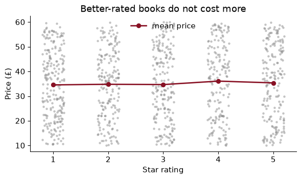
The mean price is £34.56 for one-star books and £35.37 for five-star ones, and the correlation between rating and price is 0.03. On a real retailer you would expect quality and price to be related; on a practice site whose prices were generated at random, they are not. Either way the point stands: a scraped number is only as good as your understanding of how the site produced it. Before treating a scraped price as a price, a researcher does what Cavallo did and validates it against an independent source.
Suppose one book on a page had no p.price_color element (out of print, say). What happens to the scraper above, and what would have happened if you had scraped all the titles with one select and all the prices with another, then put the two lists side by side?
In the container-first scraper, b.select_one("p.price_color") returns None and .get_text() raises an AttributeError, so the scrape stops on that book: loud, and easy to fix by checking for None and recording a missing price. In the two-lists version, the price list is one shorter than the title list, and every price after the missing one is attached to the wrong book. If the lengths happened to match up again (another book with a missing title), nothing would complain at all. This is why you select the container first: a missing field becomes a missing value in the right row, not a silent shift of every row below it.
Much of what economists want from a web page is already a table. pandas.read_html finds every <table> element in a page and returns each one as a DataFrame. Wikipedia’s list of state minimum wages is a good example: read_html with match="State" returns the 6 tables on the page that contain the word “State”.
wiki = cached_get("https://en.wikipedia.org/wiki/List_of_US_states_by_minimum_wage")
tables = pd.read_html(io.StringIO(wiki["text"]), match="State")
Fetch the page yourself rather than passing the URL to read_html. Wikipedia refuses requests without a User-Agent, and fetching it yourself lets you set headers, a timeout and a cache. Wikipedia pages also change whenever someone edits them, which is the strongest reason to save the raw HTML with its date: this copy was fetched on 2026-10-23.
The tables arrive messy, in a way that is typical of scraped tables. Each table has states down the side and two or three years across the top, so it is wide; the year headers carry footnote markers such as 2024[1][4]; state names carry asterisks; and the cells are strings like ‘$14.00 (effective July 1, 2026)’. A tidy function melts each table to long form and uses regular expressions to pull out the four-digit year and the dollar amount:
def tidy(t):
    t = t.rename(columns={t.columns[0]: "state"})
    long = t.melt(id_vars="state", var_name="year", value_name="raw")
    long["year"] = long["year"].astype(str).str.extract(r"(\d{4})")[0].astype(int)
    long["min_wage"] = long["raw"].astype(str).str.extract(r"\$(\d+\.\d+)")[0].astype(float)
    long["state"] = long["state"].str.replace(r"[^A-Za-z .]", "", regex=True).str.strip()
    return long[["state", "year", "min_wage", "raw"]]
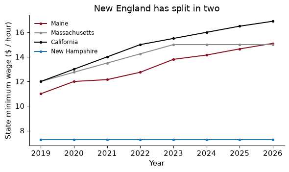
The result is a state-by-year panel from 2019 to 2026. Maine’s minimum wage rose from $11.00 to $15.10, while next door New Hampshire stayed at the federal $7.25, as do 20 states in 2026. Variation like this, across neighbouring states and over time, is the raw material of the large empirical literature on the employment effects of minimum wages.
7 cells in the scraped panel contained parentheses, like the Alaska cell above. What information did the tidy function discard, and does it matter?
print(mw.loc[mw["raw"].str.contains(r"\(", regex=True), "raw"].drop_duplicates().head(4).tolist())
['$14.00 (effective July 1, 2026)', '$16.90 (Wage by city in California)', '$15.00 (effective Sept. 30, 2026)', '$17.00 (New York City, Long Island and Westchester) $16.00 (Rest of the state)']
The regex keeps the first dollar amount and drops everything else: effective dates (“effective July 1”), notes that cities set higher wages, and sometimes a second rate for part of the state (New York City and its suburbs against the rest of New York). For a picture of the trend, that is fine. For research it is not: a wage that takes effect on July 1 is in force for half the year, and a study of teenage employment in California that uses the state rate ignores the higher city rates where many teenagers work. The scrape is a good way to check an authoritative source (the Department of Labor’s tables, or Vaghul and Zipperer’s research data set of state and local minimum wages). It is not a substitute for one.
Being able to download a page does not mean you may. There are three layers of rules, and a researcher has to respect all of them.
What the site asks. Most sites publish a file called robots.txt at their root, listing the paths that automated programs should not visit and sometimes how long to wait between requests. Python’s urllib.robotparser reads it:
rp = RobotFileParser()
rp.parse(cached_get("https://en.wikipedia.org/robots.txt")["text"].splitlines())
rp.can_fetch(ua, "https://en.wikipedia.org/wiki/Minimum_wage")
For Wikipedia, /wiki/Minimum_wage is allowed, /wiki/Special:Random is not allowed, and the search page is not allowed. books.toscrape.com has no robots.txt at all (the request returns 404), which means it states no restrictions; the site exists to be scraped. robots.txt is not a law, but ignoring it is bad practice and, if a dispute ever arises, evidence of bad faith. Read the site’s terms of service too: many prohibit scraping outright.
What the law says. I am not a lawyer and this is not legal advice, but the broad US picture is this. The Computer Fraud and Abuse Act makes it a crime to access a computer “without authorization”; Van Buren v. United States (2021) read that narrowly, and in hiQ Labs v. LinkedIn the Ninth Circuit suggested that scraping pages anyone can see without logging in is unlikely to violate it, though hiQ ultimately lost on breach of LinkedIn’s terms. Facts are not copyrightable, but text, photos and the creative selection of a database can be, so republishing what you scrape is riskier than analysing it. Logins, paywalls and CAPTCHAs are the site saying no, and getting around them is where scraping turns from research into trespass.
What ethics requires. Data about people raise questions that data about books do not. Names, profiles, photos and posts may be public and still be personal; privacy law (Europe’s GDPR, California’s CCPA) may apply; and a research project that collects them will usually need review by your college’s institutional review board. Collect only what the question needs, and think about who could be hurt if the data leaked.
Look for an API or a bulk download first. Read
robots.txtand the terms. Identify yourself, go slowly, cache everything, collect only what you need, and never get around a login.
For each, say whether you would scrape, and why. (a) Daily prices of 500 grocery products from a supermarket’s public website, to build a local price index. (b) Every public post by Maine state legislators on a social network, which requires logging in to view. (c) Rental listings from a site whose terms forbid automated access, when the site also sells the same data to researchers.
(a) Probably yes, carefully: public pages, prices are facts, no personal data, and it is the Billion Prices recipe. Check robots.txt and the terms, scrape once a day at a slow rate, cache, and validate your index against the official CPI for the region.
(b) Not by scraping. Content behind a login is the clearest “no”, and the posts are personal data even though their authors are public figures. Look for the platform’s research API or an archive that has permission, and talk to your IRB.
(c) No. The terms forbid it, and the owner offers a legitimate route. Ask for the data, or for an academic licence; many firms will say yes to a student who asks politely.
The chapter’s pipeline end to end: a cached, retrying session; a paginated API call; a keyless CSV; a scrape that follows “next” links; and a table read from a web page.
import io, json, time, hashlib, datetime as dt
from pathlib import Path
import pandas as pd, requests
from bs4 import BeautifulSoup

CACHE = Path("../data/web"); CACHE.mkdir(parents=True, exist_ok=True)
# `session` (User-Agent, retries) and `cached_get` are as defined in "Being a good citizen".
A World Bank indicator for every country, every page, aggregates removed.
school, meta = wb_get("SE.SEC.ENRR", date="2019")          # secondary school enrolment, gross %
school = school[school["countryiso3code"].isin(real)].dropna(subset=["value"])
print(f"{meta['pages']} pages, {len(school)} countries with data")
3 pages, 141 countries with data
FRED without a key, and a scrape of the whole catalogue.
fred = pd.read_csv(io.StringIO(cached_get("https://fred.stlouisfed.org/graph/fredgraph.csv",
                                          params={"id": "UNRATE,CPIAUCSL"})["text"]),
                   parse_dates=["observation_date"], index_col="observation_date")
books = scrape_books().assign(price=lambda d: d["price"].str.extract(r"(\d+\.\d+)")[0].astype(float))
assert len(books) == 1000 and books["price"].notna().all(), "the scrape did not get every book"
print(f"FRED to {fred.index.max():%Y-%m}; {len(books):,} books, median price £{books['price'].median():.2f}")
FRED to 2026-09; 1,000 books, median price £35.98
Trusting a 200. The World Bank returns “OK” with an error message for an indicator that does not exist. Check the status and the content: raise_for_status(), then an assert that you got rows.
Forgetting pagination. You get the first page, 50 or 100 records, and a perfectly plausible DataFrame. Read the metadata, loop until page >= pages, and check the row count against total.
Keeping aggregates. “All countries” includes “World”, regions and income groups. Filter them out before you count, average or regress.
Committing an API key. It is in your Git history forever. Use environment variables or .env, put .env in .gitignore first, and if a key leaks, revoke it.
Re-downloading on every run. It is slow, it is rude to the server, and it makes your results depend on whether a website is up today and what it says today. Cache raw responses with the date, and run the analysis from the cache.
Scraping fields separately, or positionally. Lists of titles and prices built by separate selects drift out of alignment the moment one record lacks a field; positional selectors break at the first redesign. Select the container, then the fields within it, with meaningful class names.
Explain the difference between a 403 and a 429 status code, and what your code should do on receiving each.
Use wb_get to download GDP per capita for the United States, China and India (countries="USA;CHN;IND") for 1990–2023 and plot the three series on a log scale. Which grew fastest?
Request the World Bank indicator for life expectancy with per_page=50 instead of 100. How many pages does the metadata report? Check that wb_get returns the same number of rows either way.
Re-draw the Preston curve, adding a fitted line of life expectancy on log GDP per capita. Which three countries lie furthest below the line, living shortest for their income?
From the scraped books, compute the share in stock and the mean price by star rating. Then explain why “the site’s prices are uncorrelated with ratings” is a statement about the site, not about books.
Using the scraped minimum-wage panel, list the states whose minimum wage rose by more than $3 an hour between the first and last year in the table. Which region are they in?
Write a function polite_get(url, last={}) that ensures at least one second passes between any two calls it makes, no matter where in your code they come from. (Hint: store the time of the last call.)
In two or three sentences: what is the representativeness problem with online prices as a measure of inflation, and how did Cavallo address it?
1. A 403 means “forbidden”: the server understood you and refuses, perhaps because your key is wrong, you lack permission, or you have been blocked. Retrying will not help; fix the key or stop. A 429 means “too many requests”: you are allowed, just not this fast. Wait (respect the Retry-After header if there is one) and retry with backoff, and slow your requests down. That is why status_forcelist in our retry policy includes 429 but not 403.
2.
three, _ = wb_get("NY.GDP.PCAP.KD", countries="USA;CHN;IND", date="1990:2023")
three = three.assign(year=lambda d: d["date"].astype(int)).dropna(subset=["value"])
growth = (three.sort_values("year").groupby("country.value")["value"]
               .agg(lambda s: (s.iloc[-1] / s.iloc[0]) ** (1 / (len(s) - 1)) - 1))
fig, ax = plt.subplots()
for (c, d), col in zip(three.groupby("country.value"), [GARNET, GREY, BLUE]):
    ax.plot(d["year"], d["value"], color=col, label=c)
ax.set_yscale("log"); ax.set(xlabel="Year", ylabel="GDP per capita (2015 US$, log)")
ax.legend(frameon=False); plt.show()
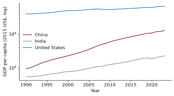
Average annual growth of GDP per capita over the period: China 8.2%, India 4.4%, United States 1.6%. China’s line is the steepest, which on a log scale means the fastest growth rate, even though the United States remains far richer in levels.
3.
life50, meta50 = wb_get("SP.DYN.LE00.IN", date="2019", per_page=50)
With 50 records a page the metadata reports 6 pages; with 100, 3. Both return 266 rows, as they must: the page size changes the number of requests, not the data. If they had differed, the loop would have a bug at the last page.
4.
b1, b0 = np.polyfit(np.log(pc_real["value_gdp"]), pc_real["value_le"], 1)
pc4 = pc_real.assign(resid=lambda d: d["value_le"] - (b0 + b1 * np.log(d["value_gdp"])))
worst = pc4.nsmallest(3, "resid")[["country.value", "value_gdp", "value_le", "resid"]]
print(worst.round(1).to_string(index=False))
           country.value  value_gdp  value_le  resid
Central African Republic      401.8      31.5  -28.3
                 Nigeria     2431.5      53.0  -15.1
                  Naoero     7687.2      61.4  -11.9
The three countries furthest below the line are Central African Republic, Nigeria, Naoero (the last is the World Bank’s spelling of Nauru), living between 12 and 28 years less than the curve predicts for their income. Each has a story that income does not capture: decades of conflict in the Central African Republic; in Nigeria, oil revenue that raises national income far more than it raises what most households live on, and high child mortality; in Nauru, a phosphate-mining fortune and some of the world’s highest rates of obesity and diabetes. The Preston curve is a description of the typical relationship; the residuals are where the interesting economics is.
5.
b5 = scrape_books().assign(stars=lambda d: d["rating"].map(stars),
                           price=lambda d: d["price"].str.extract(r"(\d+\.\d+)")[0].astype(float),
                           in_stock=lambda d: d["stock"].str.contains("In stock"))
print(b5.groupby("stars").agg(in_stock=("in_stock", "mean"), mean_price=("price", "mean")).round(2).to_string())
       in_stock  mean_price
stars
1           1.0       34.56
2           1.0       34.81
3           1.0       34.69
4           1.0       36.09
5           1.0       35.37
All 1,000 books on the catalogue pages are listed as in stock (100%), and mean prices barely vary with the rating. Both facts describe how a practice site was built (prices and ratings assigned without any market behind them), not how books are priced. Scraped data inherit the process that produced the page, which is why you validate before you interpret.
6.
rise = (mw.pivot(index="state", columns="year", values="min_wage")
          .assign(change=lambda d: d[latest_year] - d[first_year])
          .query("change > 3").sort_values("change", ascending=False))
print(rise["change"].round(2).to_dict())
{'Florida': 6.54, 'Missouri': 6.4, 'Delaware': 6.25, 'Nebraska': 6.0, 'Connecticut': 5.94, 'New Jersey': 5.92, 'Hawaii': 5.9, 'New York': 5.9, 'Illinois': 5.75, 'Virginia': 5.52, 'Rhode Island': 5.5, 'Washington': 5.13, 'Oregon': 5.05, 'Maryland': 4.9, 'California': 4.9, 'New Mexico': 4.5, 'Michigan': 4.28, 'Arizona': 4.15, 'Alaska': 4.11, 'Maine': 4.1, 'Colorado': 4.06, 'Washington D.C.': 3.95, 'Nevada': 3.75, 'Vermont': 3.64}
24 jurisdictions (D.C. is in the table) raised their minimum wage by more than $3 between 2019 and 2026. The four largest increases were in Florida, Missouri, Delaware, Nebraska. That is not the list most people would guess, and the explanation is political: Florida, Missouri and Nebraska raised their wages by ballot measure, voted on directly, rather than through the legislature. The rest are mostly in the Northeast and the West. The states that stayed at $7.25 are mostly in the South and the Plains.
7.
def polite_get(url, last={"t": 0.0}, gap=1.0, **kwargs):
    """requests.get, but never more than once per `gap` seconds."""
    wait = last["t"] + gap - time.monotonic()
    if wait > 0:
        time.sleep(wait)
    last["t"] = time.monotonic()
    return session.get(url, timeout=30, **kwargs)
The default argument last is a single dictionary shared by every call (a Python quirk that is usually a bug, and here is exactly what we want), so it remembers when the previous request was made. time.monotonic() is used rather than the wall clock because it never jumps backwards when the computer’s clock is adjusted.
8. Online prices cover only products and retailers that sell online, which in the 2000s skewed towards some categories (electronics, groceries at big chains) and away from others (services, housing, small shops), so an online index could track a different basket from the CPI. Cavallo addressed it by validating: scraping retailers that sell both online and offline, collecting in-store prices for the same products at the same time, and showing that they were identical about 72% of the time. Housing and services are still largely missing, so online price indices are best seen as a fast, high-frequency complement to the official CPI, not a replacement.
Three papers by economists who went to the web for data that no agency publishes, and thought hard about whether it measures what they wanted.
Cavallo, A. & Rigobon, R. (2016). “The Billion Prices Project: Using Online Prices for Measurement and Research.” Journal of Economic Perspectives 30(2): 151–178. doi.org/10.1257/jep.30.2.151
The story that opens this chapter, told by the people who did it. They explain how they scraped daily prices from large online retailers around the world, how they turned those prices into inflation indices, and how closely the indices track official consumer price statistics (closely in most countries, not at all in Argentina while its official figures were in doubt). They also show what else daily product-level prices let you study: how often prices change, and whether the same good costs the same in different countries.
Think about: an online index only sees products that are sold online by the retailers you chose to scrape. What kinds of spending (rent, services, small shops) does it miss, and when would that make it a poor guide to the cost of living for low-income households?
Edelman, B. (2012). “Using Internet Data for Economic Research.” Journal of Economic Perspectives 26(2): 189–206. doi.org/10.1257/jep.26.2.189
A practical tour of how economists collect data from websites, written for researchers rather than programmers. Edelman describes what can be gathered (prices, listings, reviews, auctions), how online settings make field experiments cheap, and the hazards: data that change under your feet, samples that are not representative, and the legal and ethical questions that come with automated collection. Much of it is the “rules of the road” section of this chapter, argued from experience.
Think about: a site’s terms forbid scraping, but the prices you need are visible to anyone with a browser. Who bears the costs of your scraper (the site’s servers, its competitors, its customers), and how would you decide whether collecting the data is acceptable?
Choi, H. & Varian, H. (2012). “Predicting the Present with Google Trends.” Economic Record 88(s1): 2–9. doi.org/10.1111/j.1475-4932.2012.00809.x
Official statistics such as retail sales or unemployment claims arrive with a lag; Google search volumes arrive almost immediately. Choi and Varian add search-volume indices to simple time-series forecasting models and show that they improve “nowcasts” of the current month’s value for series like car sales, travel and initial jobless claims. The data come from a web service, not from a file anyone curated for economists.
Think about: Google Trends reports an index that Google scales and samples itself, and it can revise past values. What does that mean for someone trying to reproduce a nowcast a year later, and why does caching the raw API response, as this chapter does, matter for research and not just for speed?
Reading. McKinney, Python for Data Analysis, 3rd ed. (2022), ch. 6, for JSON, HTML tables and web APIs. Mitchell, Web Scraping with Python, 3rd ed. (2024), for scraping in depth, including JavaScript pages. Cavallo and Rigobon (2016), “The Billion Prices Project”, Journal of Economic Perspectives; Cavallo (2017), “Are Online and Offline Prices Similar?”, American Economic Review; Edelman (2012), “Using Internet Data for Economic Research”, Journal of Economic Perspectives.