The question: a mobile game makes new players stop and wait (or pay) when they reach level 30. Would moving that gate to level 40 keep more of them playing a week later?
Cookie Cats is a puzzle game for phones. Like many free games, it has gates: at certain levels the player must either wait a while or pay to continue. A gate is a small piece of economic design. It slows down players who are burning through the content, it nudges some of them to spend money, and it may annoy others into deleting the game. The developer’s question is where to put the first one.
Suppose you looked at existing data and found that players who got past level 40 were much more likely to still be playing a week later. Would that tell you anything about where to put the gate? Almost nothing. Players who get far are the keen ones, and keen players come back. The comparison mixes the effect of the game’s design with the effect of who chose to keep playing.
The clean way to say this uses potential outcomes. Each player $i$ has two outcomes we could in principle see: $Y_i(1)$, whether she is still playing after a week if her gate is at level 40, and $Y_i(0)$, the same if it is at level 30. The effect of the gate on her is $Y_i(1) - Y_i(0)$. We only ever see one of the two, which is why causal inference is hard. Compare people who happened to get one version with people who happened to get the other, and
\[\text{observed gap} = \text{average effect} + \underbrace{\text{how different the two groups were anyway}}_{\text{selection bias}}\]A randomized experiment kills the second term. If a coin flip decides which version each player gets, the two groups are alike, on average, in everything: keenness, phone, country, mood. Then the simple difference in average outcomes estimates the average treatment effect (ATE), the average of $Y_i(1) - Y_i(0)$ across players. No control variables are needed, and none could do as well, because a coin flip balances the things you cannot measure too.
This is the only chapter in the book that is mainly about causation. Everything from Chapter 9 on is about prediction. But firms run experiments on a scale that would make any development economist envious. Microsoft, Amazon, Booking and Netflix run thousands a year, and their name for a randomized experiment is an A/B test: version A is the control, version B the treatment. Economists use the same design to study Medicaid (the Oregon lottery), job-search assistance, and the prices firms charge. The logic is identical; only the vocabulary differs.
A coin flip does not make the groups identical. It makes them different only by chance, and chance is something we know how to measure.
Among players with the gate at level 30, those who played at least 40 rounds in their first two weeks came back on day 7 at a rate of 50%; those who played fewer came back at 5%. A product manager concludes that “getting players to 40 rounds” would raise day-7 retention by about 45 percentage points. What is wrong?
Two things. First, selection: players who play 40 rounds are the ones who like the game, and they would have come back on day 7 whatever we did. The gap is almost entirely the second term of the equation above. Second, rounds played is itself an outcome, measured over the same two weeks as the return visit. Playing a lot and coming back are two symptoms of the same enthusiasm, not cause and effect. If you want to know what moving the gate does, you randomize the gate. Which is exactly what the developer did.
Before anyone flips a coin, three decisions have to be written down.
The unit of randomization is the thing that gets the coin flip. In Cookie Cats it is the player: each new install was assigned to gate_30 (control) or gate_40 (treatment) and kept that version. Other choices are common:
| Unit | Example | Watch out for |
|---|---|---|
| User (logged-in ID) | a new recommendation algorithm | the default; consistent experience across visits |
| Cookie or device | logged-out visitors | one person on two devices gets both versions |
| Page view | search ranking | users see both versions, so effects leak between them |
| Cluster (city, store) | delivery fees, driver pay | few units, so much less precision |
| Time period (switchback) | a surge-pricing algorithm | carry-over from one period to the next |
The rule of thumb: randomize at the level where spillovers stop, and analyse at the level you randomized. If you randomize cities, your sample size is the number of cities, not the number of riders.
Platforms do not flip coins live. They pass the user ID, combined with the experiment’s name, through a hash function, a scrambler that turns any text into a random-looking but repeatable number. The same player always gets the same version, and adding the experiment’s name keeps two experiments running at once independent of each other.
import hashlib

def assign(user_id, experiment, p_treat=0.5):
    h = hashlib.md5(f"{experiment}:{user_id}".encode()).hexdigest()
    return int(int(h[:8], 16) / 16**8 < p_treat)       # first 8 hex digits -> [0, 1)

print([assign(u, "gate_test") for u in [116, 337, 377, 483, 488]])
[0, 1, 1, 0, 0]
The metric. Experienced teams pick one overall evaluation criterion (OEC), the metric the launch decision rests on, and they pick it before they see any data. It should track long-run value. For a free game that earns money from engaged players, retention_7 (did the player open the game seven days after installing?) is a sensible OEC: it is closer to “will this player stick around” than anything measured on day one.
Guardrails are metrics that must not get worse even if the OEC improves: crash rates, page load time, refunds, complaints. A new checkout page that raises revenue by crashing on old phones is not a win. The data we have for Cookie Cats contain three outcomes, retention_1, retention_7 and sum_gamerounds (rounds played in the first 14 days), so here the guardrail role falls on engagement: moving the gate later should not make people play less.
For each experiment, choose the unit of randomization. (a) A news site tests a new headline font. (b) A ride-hailing firm tests a higher pay rate for drivers. (c) A supermarket chain tests a new shelf layout.
(a) The user (or the cookie, for logged-out readers). A font affects only the person reading it, and you want each reader to see one version consistently.
(b) Not the driver. Drivers paid more will work more hours and take rides that control drivers would have taken, so the control group is hurt by the treatment and the comparison overstates the effect. Randomize whole cities, or alternate the pay rate over time within a city (a switchback).
(c) The store. You cannot show one shopper a different shelf from the one beside her. With, say, 40 stores you have 40 units, and the power calculation later in the chapter will be sobering.
Before looking at any outcome, check that the experiment ran as designed. The Cookie Cats split was meant to be 50/50. Here is what we got:
print(cc["version"].value_counts())
version
gate_40    45489
gate_30    44700
Name: count, dtype: int64
That is 45,489 players at level 40 and 44,700 at level 30, a gap of 789 players, or 50.44% in the treatment group. It looks like a rounding error. Is it?
A fair coin tossed 90,189 times does not give exactly half heads, but it gets very close. A chi-squared test compares observed counts with the counts the design implies:
stats.chisquare([n40, n30], [n_all / 2, n_all / 2])
Power_divergenceResult(statistic=np.float64(6.9024049496058275), pvalue=np.float64(0.008607987810836243))
The $p$-value is 0.0086. If assignment really were a fair coin, a split this lopsided would happen less than once in a hundred experiments. This is a sample ratio mismatch (SRM), and it is a real one, in a famous teaching data set that most tutorials analyse without mentioning it.
Why does a small imbalance in counts matter so much? Because a coin cannot produce it, something else did, and that something may also be correlated with the outcome. Common causes in practice:
Each of these breaks the guarantee that made the experiment worth running: the two groups may no longer be comparable. The standard advice, from teams that run thousands of experiments, is blunt. An SRM means stop and debug before you trust any result. We do not have the developer’s logging code, so we cannot find the bug. What we can do is carry the warning into every conclusion below, and you will see that I do.
Hunting for the SRM’s source, a colleague counts players in each arm by the number of rounds they played:
version         gate_30  gate_40  share at 40
sum_gamerounds
0                  1937     2057        0.515
1–5               10119    10604        0.512
6–20              12428    12657        0.505
21–30              3858     3902        0.503
31–40              3070     2669        0.465
41–100             7193     7310        0.504
100+               6095     6290        0.508
She points out that among players with 31–40 rounds only 46.5% are in the level-40 group, and says she has found the bug. Has she?
No. Rounds played is an outcome of the experiment. Players whose gate is at level 30 hit it around then and many stop, so they pile up in the 31–40 bin; players with the gate at 40 keep going past it. That table shows the treatment working, not a logging fault. Slicing an SRM by a post-treatment variable mixes the two up. The places to look are things fixed before assignment: install date, app version, device, country. Our data contain none of those, which is precisely why we cannot diagnose this SRM, only report it.
With randomization doing the hard work, the estimate is the obvious one: the average outcome in the treatment group minus the average in the control group. The question that takes some thought is how much that gap would bounce around if we reran the experiment with a fresh coin. That is its standard error:
\[\hat\tau = \bar Y_{1} - \bar Y_{0}, \qquad SE(\hat\tau) = \sqrt{\frac{s_1^2}{n_1} + \frac{s_0^2}{n_0}}\]where $s_1^2$ and $s_0^2$ are the sample variances of the outcome in each group. Each group mean has its own sampling noise, $s^2/n$; the two groups are independent, so the variances add. You met this formula in intro statistics. Here is the whole of it as a function:
def diff_in_means(y, d):
    y1, y0 = y[d == 1], y[d == 0]
    est = y1.mean() - y0.mean()
    se = np.sqrt(y1.var(ddof=1) / len(y1) + y0.var(ddof=1) / len(y0))
    return est, se
For day-7 retention, 19.02% of control players came back, against 18.20% of treated players. The estimate is -0.82 percentage points, with a standard error of 0.26 points. A 95% confidence interval is the estimate plus or minus about two standard errors: from -1.33 to -0.31 points. The whole interval is below zero. Moving the gate later made players less likely to come back.
That surprises most people, so it is worth an economic story. A gate is a forced break. A player who is made to stop at level 30 may come back to it the next day; a player allowed to binge to level 40 may get bored sooner. Whatever the mechanism, the experiment answers the question it was designed to answer, and the answer is “keep the gate at 30”, with the SRM caveat attached.
Report the relative change too. A drop of 0.82 points on a base of 19.0% is a 4.3% fall in the number of players still around after a week. For a game with millions of installs, that is a lot of players.
For a 0/1 outcome the variance has a simple form, $s^2 = \hat p(1-\hat p)$ (to a very close approximation). Using only the two retention rates and the two group sizes, compute the standard error of the day-7 difference.
Exactly what the function gave. The lesson is the shape of the formula: the standard error shrinks with the square root of the sample size. Ninety thousand players sounds like a lot, and it pins the effect down to within about a percentage point either way. That is fine for a change of this size and hopeless for a change ten times smaller, which is where we will go in the section on power.
A $p$-value answers one narrow question: if the gate’s position made no difference at all, how often would random assignment alone produce a gap at least this big? For a 0/1 outcome the standard tool is the two-proportion $z$-test:
from statsmodels.stats.proportion import proportions_ztest
s7 = cc.groupby("treat")["retention_7"].agg(["sum", "count"]).loc[[1, 0]]   # treatment first
proportions_ztest(s7["sum"], s7["count"])
(np.float64(-3.164358912748191), np.float64(0.0015542499756143289))
The $z$-statistic is -3.16 and $p$ = 0.0016. For day-1 retention the gap is smaller, -0.59 points, with $p$ = 0.074: not significant at 5%. We return to why the day-1 and day-7 answers differ.
The same estimate comes out of a regression. Regress the outcome on a 0/1 treatment dummy and the coefficient on the dummy is the difference in means. Ask for robust (heteroskedasticity-consistent) standard errors, cov_type="HC1", and the standard error matches the formula above, because robust errors do not assume both groups have the same spread:
ols7 = smf.ols("retention_7 ~ treat", data=cc).fit(cov_type="HC1")
print(f"coefficient {ols7.params['treat']:.5f}, SE {ols7.bse['treat']:.5f}")
coefficient -0.00820, SE 0.00259
A $t$-test, a proportions test and OLS on a dummy are three doors into the same room. I reach for the regression because it is the one that lets you add covariates, which is the next section.
Estimate the effect on sum_gamerounds, rounds played in the first two weeks, with a regression on treat. Then look at the largest value in the data, drop it, and estimate again.
With everyone, the estimated effect is -1.16 rounds (SE 1.31, $p$ = 0.38). The largest value is 49,854 rounds in two weeks, by a player in gate_30. The next largest is 2,961. That is about 3,561 rounds a day, which is either a bot or a logging error, not a person.
Drop that one player out of 90,189 and the estimate becomes -0.04 rounds (SE 0.68), and the standard error falls by 48%. One row moved the mean of the control group by about 1.0 rounds. Means of very skewed outcomes are fragile, which is why the median (17 rounds in control, 16 in treatment) or a winsorized mean is often reported alongside. Decide your rule for outliers before you look at the results, and report both versions if they differ.
Randomization removes bias. It does not remove noise. Some players would have come back on day 7 and some would not, whatever version they got, and that player-to-player variation is what makes the standard error as large as it is. If we could predict part of it from information we had before the experiment, we could subtract the predictable part and be left with a less noisy outcome.
Cookie Cats players are new installs, so there is no “before”. Most experiments are not like that: a retailer testing a checkout page knows what each customer spent last month, and last month’s spending predicts this month’s very well. So for this section we simulate, using the setup from Exercise 12. A subscription service shows half of 20,000 users a 10% discount. We know each user’s spending last month, pre, and the true effect of the discount on spending this month is $1.50.
The adjustment, known in industry as CUPED (Controlled-experiment Using Pre-Experiment Data; Deng, Xu, Kohavi and Walker 2013), replaces each user’s outcome with
\[Y_i^{\text{adj}} = Y_i - \theta\,(X_i - \bar X)\]where $X_i$ is last month’s spend and $\theta$ is the slope from regressing $Y$ on $X$. Then compute the difference in means on $Y^{\text{adj}}$ instead of $Y$.
theta = np.cov(spend, pre)[0, 1] / np.var(pre, ddof=1)     # slope of Y on X
spend_cuped = spend - theta * (pre - pre.mean())
print(diff_in_means(spend, treat_s), diff_in_means(spend_cuped, treat_s))
(np.float64(1.9583406721881254), np.float64(0.29615082492681133)) (np.float64(1.7575749822325122), np.float64(0.1709027419737525))
| Estimate | Standard error | |
|---|---|---|
| Raw difference in means | $1.96 | 0.296 |
| CUPED | $1.76 | 0.171 |
OLS with centred pre as a control |
$1.76 | 0.171 |
Both estimates are within two standard errors of the true $1.50 (the raw one misses by more, which is what a noisier estimate does), and the CUPED standard error is much smaller: the variance of the estimate falls by 67%. The last row is the version an econometrician would write. Adding a pre-treatment covariate to the regression is CUPED, up to tiny differences in how $\theta$ is estimated. You were taught in econometrics that adding controls in an experiment is about precision, not bias; this is that lesson with a price tag attached.
Why is it safe? Because $X$ was measured before the coin was flipped, the treatment cannot have changed it, and its average is the same in both arms (randomization again). Subtracting $\theta(X - \bar X)$ therefore takes noise out of both groups without moving the gap between them. How much noise it removes depends only on how well $X$ predicts $Y$: the variance falls by a factor of $1 - \rho^2$, where $\rho$ is their correlation. Here $\rho$ = 0.82, so theory says a reduction of 67%, which is what we got.
Controls in an experiment buy precision, not unbiasedness. Use only controls the treatment cannot have touched.
Going further. The variance of $Y - \theta X$ is $\text{Var}(Y) - 2\theta\,\text{Cov}(Y,X) + \theta^2\text{Var}(X)$. Minimise over $\theta$ and you get $\theta = \text{Cov}(Y,X)/\text{Var}(X)$, the OLS slope, and a minimised variance of $(1-\rho^2)\text{Var}(Y)$. Freedman (2008) showed that plain regression adjustment can occasionally hurt precision in experiments with unequal group sizes; Lin (2013) showed that interacting the treatment with the centred covariate (spend ~ treat * pre_c) fixes this, and is never worse in large samples.
The CUPED-adjusted analysis has 67% less variance than the raw one. How many users would the raw analysis need to be as precise as CUPED on 20,000?
Variance of a mean is proportional to $1/n$. Cutting the variance by a share $v$ is the same as multiplying the sample by $1/(1-v)$: here $1/(1 -$ 0.67$)$ ≈ 3.0. The raw analysis would need about 60,056 users. CUPED gets you those extra users free, from data you already had. That is why every large experimentation platform does it, and why the most valuable thing a firm can log about its customers is often their behaviour before the test.
Every experiment should be sized before it starts. Three numbers set the size:
For a two-arm test with $n$ users per arm, $\alpha = 0.05$ and 80% power, a good approximation is
\[\text{MDE} \approx 2.8 \times \sigma \times \sqrt{2/n}\]where $\sigma$ is the standard deviation of the outcome. (The 2.8 is 1.96 for the test plus 0.84 for the power.) For a 0/1 outcome, $\sigma = \sqrt{p(1-p)}$.
Two things follow from the square root, and they explain most of what you will hear about experiments in industry. Halving the MDE takes four times the users. And anything that cuts $\sigma$ cuts the MDE directly, which is CUPED’s real value: a variance reduction of half is worth the same as doubling the experiment.
For Cookie Cats, the baseline day-7 retention is 19.0%. With about 45,000 players per arm the formula gives an MDE of 0.73 percentage points (the exact calculation in statsmodels gives 0.73). The effect we found, 0.82 points, is just above it, so the experiment was big enough, but not by much.
from statsmodels.stats.power import NormalIndPower
from statsmodels.stats.proportion import proportion_effectsize
h_half = proportion_effectsize(0.19, 0.185)            # 19% -> 18.5%
NormalIndPower().solve_power(effect_size=h_half, alpha=0.05, power=0.8)
95654.16347346478
To detect a drop of half a point, from 19% to 18.5%, needs 95,654 players per arm. To detect a 1% relative change, from 19% to 18.81%, needs 666,650 per arm, over 1 million players. This is why Google can test the shade of blue in a link and a small firm cannot: small firms should test bold changes, because only bold changes are detectable with the traffic they have.
A small studio has 3,000 new players a week and runs a gate experiment for one week. The true effect is the one we estimated, about 0.8 points. What is the power of their test, and what does a “significant” result from it look like?
With 1,500 per arm, simulating 20,000 such experiments, only 9% come out significant. That is the power: the studio will usually conclude “no effect”. Worse, the experiments that do reach significance are the ones where noise happened to push the estimate far from zero. Among them, the average estimated effect is 4.1 times the true effect. An underpowered experiment that “works” exaggerates. This is the winner’s curse, and it is one reason published effects in economics and psychology shrink when someone replicates them.
Dashboards update every morning. The product manager looks at the $p$-value each day and stops the experiment the first time it drops below 0.05. What could be wrong with that?
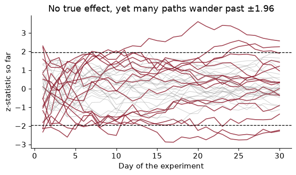
Simulate it. Run 1,000 A/A tests, experiments in which both arms get the same game, so that every “significant” result is a false positive. Each runs for 30 days, with 300 new players per arm per day and a true retention rate of 19% in both. After each day, compute the $z$-statistic on all the data so far.
rng = np.random.default_rng(368)
sims, days, per_day, p0 = 1_000, 30, 300, 0.19
x1 = rng.binomial(per_day, p0, (sims, days)).cumsum(axis=1)   # retained so far, arm 1
x0 = rng.binomial(per_day, p0, (sims, days)).cumsum(axis=1)
n_cum = per_day * np.arange(1, days + 1)
p_pool = (x1 + x0) / (2 * n_cum)
z = (x1 / n_cum - x0 / n_cum) / np.sqrt(p_pool * (1 - p_pool) * 2 / n_cum)
sig = np.abs(z) > 1.96
print(sig[:, -1].mean(), sig.any(axis=1).mean())
0.053 0.301
Look only on day 30 and 5.3% of the A/A tests are significant, close to the promised 5%. Look every day and stop at the first significant result, and 30% are. The test’s 5% guarantee holds for one look. Thirty looks give the noise thirty chances.
The $z$-statistic is a random walk that has been scaled to stay put on average. Wait long enough and it wanders across any fixed line. The fixes:
The manager stopped an experiment on day 4 with $p$ = 0.03, and the estimated lift was large. You ran the same A/A simulation. How would you explain to her why you do not believe the result?
The $p$-value of 0.03 is computed as if day 4 had been chosen in advance. It was not: she would have stopped on any day the $p$-value happened to dip, so the real false positive rate of her procedure is the 30% in the simulation, not 5%. And the effect estimate is biased upwards too: an experiment stopped at the first lucky dip is stopped precisely when noise is flattering the treatment. The fix is not to argue; it is to rerun the test, pre-registering a sample size, and look once.
A real experimentation dashboard reports dozens of metrics. Suppose a change does nothing at all, and you test 20 independent metrics at the 5% level. Simulating 5,000 such experiments, at least one metric is “significant” in 65% of them. (The arithmetic: $1 - 0.95^{20} \approx 0.64$.) Every dashboard has a green number on it somewhere.
There are two standard corrections:
Here are five Cookie Cats metrics, with raw and adjusted $p$-values:
                            p  Bonferroni     BH
retention_1            0.0744      0.3720 0.1860
retention_7            0.0016      0.0078 0.0078
mean rounds            0.3759      1.0000 0.4699
share with 0 rounds    0.1686      0.8429 0.2810
share with 100+ rounds 0.4971      1.0000 0.4971
Day-7 retention survives both corrections (Bonferroni 0.008, BH 0.008). The others do not reach 5% after correction. But the best defence against multiple testing is not a formula, it is the discipline from the start of the chapter: name one OEC before the experiment, and treat every other metric as a diagnostic that helps you understand the result rather than as a second chance to find one.
The same applies to segments. “The treatment did nothing overall but it worked for Android users in Brazil on weekends” is a multiple-testing result until a new experiment confirms it.
With the five metrics above, what threshold does Bonferroni set, and which raw $p$-values clear it?
The threshold is 0.05 / 5 = 0.01. Only retention_7, with raw $p$ = 0.0016, is below it. Equivalently, multiply each $p$-value by 5 (capping at 1) and compare with 0.05, which is what the “Bonferroni” column shows. retention_1, with $p$ = 0.074, was not significant even before the correction.
Two last problems have nothing to do with statistics and everything to do with people.
People react to change itself. A new button gets clicked because it is new, and the clicks fade over a few weeks (novelty). A new layout annoys experienced users until they learn it, and the effect improves over time (primacy). A two-week experiment can measure either and call it the long-run effect. The fix is to plot the estimated effect by day since exposure and run long enough to see where it settles, or to look separately at new users, who have no old habits to break.
Cookie Cats gives a related warning. On day 1 the difference between the arms is -0.59 points and not significant; by day 7 it is -0.82 and clearly significant. That makes sense: most players do not reach level 30 on their first day, so on day 1 the two versions of the game are nearly identical. A team that judged the experiment on day-1 retention might well have called the change harmless and shipped it. The metric’s time horizon has to match when the treatment can bite.
My treatment can affect your outcome. The analysis assumes each player’s outcome depends only on her own version. Econometricians call this SUTVA, the stable unit treatment value assumption, or more plainly “no spillovers”. A single-player puzzle game comes close to satisfying it. Many settings do not:
The design fix is the one from the unit-of-randomization table: randomize whole clusters (cities, network communities) or alternate over time. Both buy less bias with less precision, which is a trade worth making when the bias is large.
A food-delivery app randomly gives half its customers in a city a $2 lower delivery fee. Orders from treated customers rise 15% relative to control. The app has a fixed number of couriers in each city. Is 15% what a city-wide fee cut would deliver?
Probably not. Treated customers’ extra orders occupy couriers, so control customers face longer waits and order less. Part of the 15% gap is control customers being pushed down, not treated customers being lifted up. A city-wide cut would lift everyone’s demand while couriers stay fixed, so waits would rise for all and the real effect would be smaller. The fix is to randomize cities, or hours of the day within a city, so that treated and control customers do not compete for the same couriers. Expect far fewer units and much wider confidence intervals, and say so in the power calculation.
The full analysis of the Cookie Cats experiment, runnable top to bottom.
from pathlib import Path
import numpy as np, pandas as pd
from scipy import stats
import statsmodels.formula.api as smf
from statsmodels.stats.proportion import proportions_ztest, confint_proportions_2indep
from statsmodels.stats.multitest import multipletests

path = Path("../data/cookie_cats.csv")              # download once, then reuse
if not path.exists():
    path.parent.mkdir(exist_ok=True)
    pd.read_csv(URL).to_csv(path, index=False)
cc = pd.read_csv(path)
cc["treat"] = (cc["version"] == "gate_40").astype(int)
cc[["retention_1", "retention_7"]] = cc[["retention_1", "retention_7"]].astype(int)
Step 1, before any outcome: the sample ratio check.
counts = cc["treat"].value_counts()
srm_p = stats.chisquare(counts, [len(cc) / 2] * 2).pvalue
print(f"treatment {counts[1]:,}, control {counts[0]:,}, SRM p = {srm_p:.4f}")
treatment 45,489, control 44,700, SRM p = 0.0086
Step 2: the effect on each retention metric, with a confidence interval and a $z$-test.
rows = {}
for col in ["retention_1", "retention_7"]:
    s = cc.groupby("treat")[col].agg(["sum", "count"]).loc[[1, 0]]
    z, p = proportions_ztest(s["sum"], s["count"])
    lo, hi = confint_proportions_2indep(*s.loc[1], *s.loc[0])
    rate = s["sum"] / s["count"]
    rows[col] = {"control": rate[0], "treatment": rate[1], "diff (pp)": 100 * (rate[1] - rate[0]),
                 "CI low": 100 * lo, "CI high": 100 * hi, "p": p}
print(pd.DataFrame(rows).T.round(4))
             control  treatment  diff (pp)  CI low  CI high       p
retention_1   0.4482     0.4423    -0.5905 -1.2392   0.0582  0.0744
retention_7   0.1902     0.1820    -0.8201 -1.3282  -0.3121  0.0016
Step 3: the same day-7 effect as a regression with robust standard errors, and the engagement guardrail with and without the 50,000-round player.
for name, data in [("all", cc), ("drop max", cc[cc.sum_gamerounds < cc.sum_gamerounds.max()])]:
    f7 = smf.ols("retention_7 ~ treat", data=data).fit(cov_type="HC1")
    fr = smf.ols("sum_gamerounds ~ treat", data=data).fit(cov_type="HC1")
    print(f"{name:8s} retention_7 {f7.params['treat']:+.4f} ({f7.bse['treat']:.4f}) | "
          f"rounds {fr.params['treat']:+.2f} ({fr.bse['treat']:.2f})")
all      retention_7 -0.0082 (0.0026) | rounds -1.16 (1.31)
drop max retention_7 -0.0082 (0.0026) | rounds -0.04 (0.68)
Step 4: correct the family of five metrics.
def prop_p(col):
    s = cc.groupby("treat")[col].agg(["sum", "count"]).loc[[1, 0]]
    return proportions_ztest(s["sum"], s["count"])[1]
cc["zero_rounds"] = (cc["sum_gamerounds"] == 0).astype(int)
cc["rounds_100"] = (cc["sum_gamerounds"] >= 100).astype(int)
g1, g0 = cc.loc[cc.treat == 1, "sum_gamerounds"], cc.loc[cc.treat == 0, "sum_gamerounds"]
pv = pd.Series({c: prop_p(c) for c in ["retention_1", "retention_7", "zero_rounds", "rounds_100"]})
pv["mean rounds"] = stats.ttest_ind(g1, g0, equal_var=False).pvalue
print(pd.DataFrame({"p": pv, "BH": multipletests(pv, method="fdr_bh")[1]}).round(4))
                  p      BH
retention_1  0.0744  0.1860
retention_7  0.0016  0.0078
zero_rounds  0.1686  0.2810
rounds_100   0.4971  0.4971
mean rounds  0.3759  0.4699
The recommendation I would write to the developer: keep the gate at level 30. Moving it to 40 lowered day-7 retention by about 0.8 percentage points, from 19.0% to 18.2% (95% CI -1.3 to -0.3), and did not raise engagement. But the two arms are not the 50/50 split the design promised (p = 0.009), so before relying on this I would want the assignment and logging code checked, and ideally a rerun.
Skipping the SRM check. It takes one line, and it is the most common reason an experiment’s result is wrong. The Cookie Cats split is off by less than one percentage point, which is invisible to the eye and very visible to a chi-squared test. Run it before you look at any outcome, and if it fails, find the cause before you report anything.
Peeking and stopping on significance. Looking every day and stopping at the first $p < 0.05$ turned a 5% false positive rate into 30% in our simulation. Fix the sample size in advance, or use a sequential method built for repeated looks.
Controlling for something the treatment affected. CUPED works because pre was measured before assignment. Add sum_gamerounds as a “control” in the retention regression and you are comparing players who played the same amount, which the gate itself changed; the estimate stops meaning anything (Exercise 3). Only pre-treatment covariates go on the right-hand side.
Fishing across metrics and segments. Twenty metrics give a 65% chance of at least one false win. Name one OEC in advance, correct the rest, and confirm surprising segment results with a new experiment.
Running an underpowered test. A small experiment usually finds nothing, and when it does find something the estimate is exaggerated. Do the power calculation first; if the MDE is larger than any plausible effect, do not run the test, or make the change bolder.
Judging on a metric that cannot see the effect yet. Day-1 retention could not show a gate that most players had not yet reached. Choose a metric, and a duration, that match when the treatment can act, and watch for effects that fade (novelty) or grow (primacy).
The Cookie Cats SRM test gives $p \approx$ 0.009. Which of these is right? (a) The treatment caused 789 extra players to install. (b) There is a 0.9% chance the randomization worked. (c) If assignment were a fair 50/50 coin, a split this uneven would occur in under 1% of experiments. (d) The retention results are wrong. Explain what is wrong with each of the others.
Using diff_in_means, compute the day-1 retention effect, its standard error and a 95% confidence interval. Check the interval against confint_proportions_2indep.
A colleague estimates retention_7 ~ treat + sum_gamerounds “to control for engagement”. Run it. What happens to the treatment coefficient, and why is this regression the wrong one?
In the CUPED simulation, make last month’s spend a much weaker predictor: generate spend = 0.2 * pre + 1.5 * treat + rng.normal(0, 12, n). Predict the variance reduction from $\rho^2$ before computing it, then check.
Rerun the peeking simulation, but let the manager look only three times, on days 10, 20 and 30. What is the false positive rate now? What does this suggest about a compromise between looking once and looking every day?
The developer wants to plan an experiment on day-1 retention (baseline 44.8%). How many players per arm does it need to detect a 1 percentage point drop with 80% power at $\alpha = 0.05$? Why does it need fewer than an experiment on a 0.5-point drop in day-7 retention?
Winsorize sum_gamerounds at its 99th percentile and re-estimate the effect on rounds. Compare with the estimates with and without the top player. Which would you report?
1. (c). A $p$-value is a statement about how surprising the data would be if the null hypothesis held, here a fair 50/50 assignment. (a) confuses the count of players with an outcome: the gate cannot make people install the game, since installation happens before anyone sees a gate. (b) inverts the $p$-value: it is not the probability that the null is true. (d) goes too far: an SRM means the results might be biased and cannot be trusted until the cause is found, not that they are known to be wrong.
2.
y1d = cc["retention_1"].to_numpy()
e1, se1 = diff_in_means(y1d, cc["treat"].to_numpy())
s = cc.groupby("treat")["retention_1"].agg(["sum", "count"]).loc[[1, 0]]
lo_c, hi_c = confint_proportions_2indep(*s.loc[1], *s.loc[0])
print(f"{e1:.5f}  SE {se1:.5f}  CI [{e1 - 1.96 * se1:.5f}, {e1 + 1.96 * se1:.5f}]  "
      f"statsmodels [{lo_c:.5f}, {hi_c:.5f}]")
-0.00591 SE 0.00331 CI [-0.01239, 0.00058] statsmodels [-0.01239, 0.00058]
The day-1 effect is -0.59 percentage points with a standard error of 0.33, so the 95% interval runs from -1.24 to 0.06 points. It includes zero. The statsmodels interval, -1.24 to 0.06, agrees to the fifth decimal place: for a 0/1 outcome the two calculations are the same formula.
3.
bad = smf.ols("retention_7 ~ treat + sum_gamerounds", data=cc).fit(cov_type="HC1")
print(bad.params["treat"], bad.bse["treat"])
-0.007556379047811762 0.0024209187030171573
The treatment coefficient becomes -0.76 points, against -0.82 without the control. It happens not to move much here, but that is luck, not a reason to trust it. Rounds played is an outcome of the experiment: the gate changes how much people play. Conditioning on it compares a treated player and a control player who played the same number of rounds, but those are different kinds of player in the two arms, because the gate put them there by different routes. The coefficient is no longer the effect of anything. Randomization protects the simple comparison; adding a post-treatment control throws that protection away.
4.
rng = np.random.default_rng(SEED)
pre4 = rng.gamma(2, 15, n_sim)
t4 = rng.binomial(1, 0.5, n_sim)
spend4 = 0.2 * pre4 + 1.5 * t4 + rng.normal(0, 12, n_sim)
th4 = np.cov(spend4, pre4)[0, 1] / np.var(pre4, ddof=1)
_, se_a = diff_in_means(spend4, t4)
_, se_b = diff_in_means(spend4 - th4 * (pre4 - pre4.mean()), t4)
rho4 = np.corrcoef(spend4, pre4)[0, 1]
print(f"rho^2 = {rho4**2:.3f}, variance reduction = {1 - (se_b / se_a)**2:.3f}")
rho^2 = 0.117, variance reduction = 0.117
Now $\rho$ = 0.34, so $\rho^2$ predicts a variance reduction of 12%, and the simulation gives 12%. CUPED is never harmful in a large sample, but it is only as good as the covariate. A weak predictor buys little.
5.
looks = [9, 19, 29]                                   # columns for days 10, 20, 30
fp3 = sig[:, looks].any(axis=1).mean()
print(f"three looks: {fp3:.3f}  vs one look {fp_end:.3f}  vs daily {fp_peek:.3f}")
three looks: 0.113 vs one look 0.053 vs daily 0.301
With three looks the false positive rate is 11.3%: worse than one look (5.3%), much better than thirty (30.1%). A few pre-planned looks cost something, and the cost can be paid by using a stricter threshold at each look. That is exactly what group-sequential designs do: they spend the 5% across a few scheduled interim analyses.
6.
b1 = r1[0]
n_r1 = NormalIndPower().solve_power(effect_size=proportion_effectsize(b1, b1 - 0.01),
                                    alpha=0.05, power=0.8)
print(f"{n_r1:,.0f} per arm, vs {n_half:,.0f} per arm for 0.5 pp on day 7")
38,736 per arm, vs 95,654 per arm for 0.5 pp on day 7
About 38,736 players per arm. That is fewer than the 95,654 needed for a half-point drop in day-7 retention because the target effect is twice as large (and sample size scales with one over the effect squared, so that alone divides it by four), even though the outcome is noisier: a 0/1 variable with a mean near 45% has a larger standard deviation, $\sqrt{0.45 \times 0.55} \approx 0.50$, than one near 19%, $\sqrt{0.19 \times 0.81} \approx 0.39$.
7.
cap = cc["sum_gamerounds"].quantile(0.99)
win = smf.ols("rounds_w ~ treat", data=cc.assign(rounds_w=cc["sum_gamerounds"].clip(upper=cap))
              ).fit(cov_type="HC1")
print(cap, win.params["treat"], win.bse["treat"])
493.0 -0.28191819808638735 0.5608352812894053
Capping at the 99th percentile (493 rounds) gives an effect of -0.28 rounds (SE 0.56), against -1.16 with everyone and -0.04 without the top player. The winsorized estimate is the one I would report, with the others in a footnote: it does not hinge on one implausible row, and it uses a rule I could have written down before seeing the data, which dropping “the player who looks odd” is not. None of the three suggests that a later gate raised engagement.
Online experiments have changed how economists study advertising and markets. These papers show what a large randomized test can overturn, and how hard it can be to detect an effect that is real.
Blake, T., Nosko, C. & Tadelis, S. (2015). “Consumer Heterogeneity and Paid Search Effectiveness: A Large-Scale Field Experiment.” Econometrica 83(1): 155–174. doi.org/10.3982/ecta12423
eBay spent heavily on search-engine ads, and its own data showed that people who clicked the ads bought a lot. The authors ran experiments, switching some of the ads off (on some search engines, and in randomly chosen local markets), and found that ads on searches for the brand name “eBay” did almost nothing: users who would have clicked the ad simply clicked the free link below it. Ads on other searches did affect infrequent and new customers, but frequent buyers, who make up most of the sales, would have come anyway. The return on the spending was far lower than the observational numbers suggested.
Think about: this is the “players who pass level 40” mistake in a business with real money at stake. Why does the correlation between seeing an ad and buying overstate the ad’s effect, and why would the bias be largest for the most loyal customers?
Lewis, R. A. & Rao, J. M. (2015). “The Unfavorable Economics of Measuring the Returns to Advertising.” Quarterly Journal of Economics 130(4): 1941–1973. doi.org/10.1093/qje/qjv023
The authors study a large set of randomized online display-ad campaigns at major retailers. The problem they document is power. Individual spending is so variable, and the effect of any one campaign so small relative to it, that even experiments with very large samples often cannot tell a campaign that pays for itself from one that loses money. It is the minimum detectable effect section of this chapter with millions of users and a disappointing answer.
Think about: Cookie Cats measures a yes-or-no outcome; a retailer measures spending, which is mostly zeros with a few very large values. Using the chapter’s formula for the minimum detectable effect, explain why the noisier outcome needs so many more users, and why a firm might keep paying for ads it can never prove work.
Athey, S. & Imbens, G. W. (2017). “The State of Applied Econometrics: Causality and Policy Evaluation.” Journal of Economic Perspectives 31(2): 3–32. doi.org/10.1257/jep.31.2.3
A readable survey of the tools economists use to estimate causal effects, with randomized experiments as the benchmark and quasi-experimental designs (regression discontinuity, difference-in-differences, synthetic controls) as the substitutes when randomizing is impossible. The authors also stress supplementary analyses, such as placebo tests and checks on robustness, which play the role that the sample ratio check plays here, and they discuss how machine learning can help find which groups respond most to a treatment.
Think about: moving a gate in a game is cheap to randomize. Pick a policy question where randomizing is impossible or unethical (raising a state’s minimum wage, say), choose one of the paper’s designs for it, and state what assumption has to stand in for the coin flip.
Reading. Kohavi, Tang & Xu (2020), Trustworthy Online Controlled Experiments, chs. 1–3 for the practice of online experiments and ch. 21 on sample ratio mismatch. Deng, Xu, Kohavi & Walker (2013) for CUPED. Angrist & Pischke (2009), Mostly Harmless Econometrics, ch. 2, for potential outcomes and why randomization works. Athey & Imbens (2017), “The Econometrics of Randomized Experiments”, for regression adjustment and design. Problem Set 3 applies all of this to a real email experiment (Hillstrom’s MineThatData data).