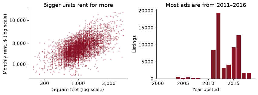
The question: a two-bedroom flat in the Bay Area comes on the market. Before anyone posts an ad, what will it rent for, and how far off is that guess likely to be?
You have spent several econometrics courses learning to estimate a coefficient. Does a year of schooling raise wages, and by how much? Does a minimum wage cost jobs? The thing you want is $\hat\beta$, and everything you were taught (unbiasedness, standard errors, identification, the omitted variable you lie awake about) is in service of getting $\hat\beta$ right.
Machine learning is for a different job. It wants $\hat y$: given what I know about this case, what is my best guess of the outcome? Nobody cares whether the coefficient on square footage is “causal”. They care whether the predicted rent is close to the rent.
Mullainathan and Spiess (2017) put this better than anyone, and their paper is the one piece of reading I would make compulsory if I could. Their point is that these are not two flavours of the same activity. Many very different models predict almost equally well. One uses bedrooms, another uses square feet, a third uses both with a wiggle; the predictions agree and the coefficients do not. So if you fit a flexible model and then read its coefficients as if they told you how the world works, you are reading tea leaves. Prediction models are judged on predictions, and only on predictions.
Why should an economist care about $\hat y$ at all? Because a surprising number of decisions need nothing else. Kleinberg, Ludwig, Mullainathan and Obermeyer (2015) call them prediction policy problems. Their example is the umbrella. Whether to take one depends on the chance of rain; it does not depend on the causal effect of umbrellas on rain, and no rain dance enters into it. A judge deciding bail needs the risk that a defendant reoffends if released. A doctor deciding on a hip replacement for an elderly patient needs to know whether the patient will live long enough to benefit. A welfare programme that wants to target the poor needs household consumption, predicted from the handful of things a survey can cheaply measure.
None of these is a causal question. All of them are economics, because each one is a decision with costs and benefits, and the prediction is only the input.
If the decision changes when $\hat\beta$ changes, you need econometrics. If the decision changes only when $\hat y$ changes, you need a good predictor, and this part of the book.
For each question, say whether it is a $\hat\beta$ problem or a $\hat y$ problem.
(a) A city wants to know whether rent control in 1994 reduced the supply of rental housing.
(b) A housing office must estimate the market rent of 3,000 units for a voucher programme, none of which has been listed.
(c) A landlord asks what an extra bedroom adds to rent, so she can decide whether to convert a study.
(d) A platform wants to flag ads whose asking rent is suspiciously far below what similar units rent for, because those are often scams.
(a) $\hat\beta$. It asks what would have happened without the policy. That is a counterfactual, and it needs a research design, not a better predictor.
(b) $\hat y$. The office does not care why a unit rents for what it does. It needs a number close to the truth for each unit.
(c) $\hat\beta$, even though it sounds like a prediction. “What does a bedroom add” is the effect of changing one thing while holding the unit otherwise fixed. A prediction model trained on listings tells you that units with more bedrooms rent for more, but those units are also bigger, newer and in different places. Converting a study changes the bedroom count without changing any of that.
(d) $\hat y$. The flag compares the asking rent with a prediction, and a large gap is the signal. Nothing causal is needed.
The trap is (c). The words “what does X add” are a causal question in disguise, and a prediction model will happily give you a confident, wrong answer to it.
Machine learning is a big tent, and it helps to know which part of it you are standing in. I sort methods along three lines.
Supervised or not. In supervised learning you have past cases where you observed the outcome, the label $y$, along with the features $x$, and you learn a rule from features to label. If the label is a number (rent, a wage, GDP next quarter) it is regression. If it is a category (default or repay, cancel or show up) it is classification, which is Chapter 12. In unsupervised learning there is no label: you look for structure in $x$ alone, such as groups of similar counties (clustering, Chapter 17) or a few indices that summarise many variables (Chapter 16). There is a third family, reinforcement learning, where an agent learns by acting and being rewarded; it matters for pricing algorithms and robots, and we will barely touch it.
Batch or online. A batch learner is trained once on a fixed data set and then used. An online learner updates as each new observation arrives. Everything in this course is batch. Online learning matters when the world drifts faster than you can retrain, as with fraud or ad auctions.
Model-based or instance-based. A model-based learner compresses the training data into a few parameters (a regression line is the obvious case) and then throws the data away. An instance-based learner keeps the training data and predicts a new case by comparing it with stored ones. The nearest-neighbour method later in this chapter is the cleanest example: to price a flat, find the most similar flats you have seen and average their rents.
Place each task on all three lines.
(a) Predict whether a loan applicant will default, from a bank’s file of past loans, retrained every quarter.
(b) Group 3,000 US counties into “types” using 40 economic indicators.
(c) Predict tomorrow’s electricity demand, updating the model every hour as new meter readings arrive, by averaging demand on the ten most similar past days.
(a) Supervised (past defaults are observed), classification (the label is yes/no), batch (retrained on a schedule, not continuously). Model-based or instance-based depends on the method; a logistic regression would be model-based.
(b) Unsupervised: there is no label, only features. Batch. Clustering methods such as k-means are model-based in the sense that they summarise the data by a few centres.
(c) Supervised regression, online (it updates every hour), and instance-based: it predicts by finding similar stored days.
Every project in Part III of this book follows the same eight steps. I will name them now and spend the rest of the chapter on one project that walks through all of them.
Steps 3 and 8 are the ones people skip, and they are the ones that make the difference between a result and a hope.
Our data are 200,796 Craigslist rental ads from the San Francisco Bay Area, 2000 to 2018, collected by Kate Pennington (2018) and distributed by TidyTuesday. Each ad has a monthly asking rent, the number of bedrooms and bathrooms, square footage, a neighbourhood, a city, a county, a date, and the free-text title of the ad.
Who would want a rent prediction, and for what?
All three want a number close to the truth, and all three are hurt more by a big miss than by a small one. That points to the loss we will use, the root mean squared error:
\[\text{RMSE} = \sqrt{\frac{1}{n}\sum_{i=1}^n (y_i - \hat y_i)^2}\]| Square each miss, average, take the square root. The square root puts it back in dollars, so an RMSE of $700 reads as “a typical miss is about $700 a month”. Squaring makes one miss of $2,000 count as much as four misses of $1,000, which is what a housing office budgeting for vouchers should want. If every dollar of error were equally bad, whatever the size of the miss, you would use the mean absolute error instead, the average of $ | y_i - \hat y_i | $. |
A model predicts three flats at $2,000, $3,000 and $2,500. They actually rent for $2,200, $2,600 and $2,500. Compute the RMSE and the MAE.
The misses are $+200$, $-400$ and $0$. Squared: 40,000, 160,000 and 0, which average to 66,667. The square root is $258.
The MAE is $(200 + 400 + 0)/3 =$ $200.
The RMSE is larger because the $400 miss was squared before it was averaged. RMSE is never smaller than MAE, and the gap between them grows when a few misses are much larger than the rest.
Before fitting anything, I look. The first thing to notice is that square footage is missing from 68% of ads. A rent model without size is not worth much, so I follow the cleaning from Exercises 13 and 18: keep whole units (not a room in a shared flat) with bedrooms, square footage and county recorded, and drop the implausible (more than five bedrooms, under 200 or over 5,000 square feet, rent under $500 or over $15,000).
That leaves 62,129 listings across 10 counties and 154 neighbourhoods. The most common county is Santa Clara, with 17,987 ads. Bathrooms are still missing for 77% of them, which we will have to deal with.
The median rent is $2,300 and the mean is $2,592. Mean above median: a right skew, a long tail of very expensive places. That tail will dominate a squared-error loss, because the biggest misses happen there.
Two things in that picture will matter later. The left panel is a cloud around a rising line, so size alone gets us a long way but leaves a lot unexplained; location and time will have to do the rest. The right panel says that 92% of the ads are from 2011 to 2016. A model trained here will know a great deal about 2012 and very little about 2005 or 2018, and no amount of cleverness changes that.
The housing office says: “Just predict the typical rent for everyone.” Which typical rent, the mean or the median, gives the lower RMSE? Which gives the lower MAE?
The mean minimises squared error and the median minimises absolute error; that is a fact about the two statistics, not about rents. On these data:
| Predict everyone at | RMSE | MAE |
|---|---|---|
| the mean, $2,592 | $1,372 | $949 |
| the median, $2,300 | $1,403 | $915 |
Each wins on its own loss. The difference is small here, but the lesson is not: the loss you choose quietly chooses the “right” answer for you, so choose it from the decision, not from habit.
The next step is the one that protects you from yourself. Before fitting anything, put a fifth of the listings aside as a test set: 12,426 ads, leaving 49,703 for training. Then do not look at it again until the very end.
from sklearn.model_selection import train_test_split
num, cat = ["sqft", "beds", "baths", "year"], ["county", "nhood"]
X, y = d[num + cat], d["price"]
X_train, X_test, y_train, y_test = train_test_split(X, y, test_size=0.2, random_state=368)
Why so strict? Because the test set is your only estimate of how the model will do on listings it has never seen, and that estimate is honest only if nothing about the model was chosen by looking at it. Every time you check the test score, try a change, and check again, a little of the test set leaks into your choices. Do it twenty times and you have fitted the test set, by hand, slowly. The score you then report is the score of the best of twenty tries, and the best of twenty is lucky by construction.
Kleinberg et al. (2018), in their study of bail decisions in New York, kept a “lock box”: a sample nobody on the team touched until the analysis was written. That is the attitude. In this course the rule is simpler: the test set is touched once, at step 8, for the one model you have already chosen.
So how do we compare models in the meantime? On the training data alone, by cross-validation, which is coming shortly.
Suppose you have twenty models that are, in truth, equally good: each would have an RMSE of exactly $750 on the whole population of future listings. You score all twenty on the same test set and report the best. Roughly what do you report?
Each test score is the truth plus some noise, because the test set is one sample. How noisy? Score even the dumbest model on five different fifths of our training data and its RMSE moves around with a standard deviation of about $13. Simulate twenty such scores, keep the smallest, and repeat ten thousand times: the reported “best” averages $726, about $24 better than any model really is.
None of the twenty is better than the others. You would be reporting luck, and calling it a finding. That is the whole case for touching the test set once.
Before any real model, I want a number to beat. The dumbest reasonable rule is to ignore the features and predict the training median, $2,300, for every flat. scikit-learn calls this a DummyRegressor, and it has the same fit and predict as any other model.
from sklearn.dummy import DummyRegressor
from sklearn.model_selection import KFold, cross_val_score
cv = KFold(5, shuffle=True, random_state=368)
base = -cross_val_score(DummyRegressor(strategy="median"), X_train, y_train,
                        cv=cv, scoring="neg_root_mean_squared_error")
Its cross-validated RMSE is $1,403. Every model that follows has to come in below that, by a margin that matters, or it is not worth the trouble.
A baseline does two jobs. It tells you whether the features carry any information at all. And it gives your reader a scale: “$700” means nothing in isolation, but “half the error of guessing the median” means a lot. Write the baseline into every table you report.
The housing office has a budget for 3,000 vouchers and sets each one at the predicted rent. If it used the median for every unit, what is a typical miss per unit, and what is that as a share of the median rent?
The typical miss is the RMSE, $1,403 a month. As a share of the median rent of $2,300 that is 61%. A voucher set that badly would be far too generous for a studio in Vallejo and hopeless for a family flat in San Francisco. We can do better than that, and the next sections will.
Here is a column I have not mentioned: the title of each ad. A few of them, cut to sixty characters:
$1425 / 1br - 735ft² - BEST LOCATION SOUTHSHORE GARDENS APAR
$3900 / 5br - 2581ft² - Gorgeous Restored Victorian - Spacio
Nov  2 Newly remodeled 4br/3ba (2 mastersuites) in quiet Fre
Craigslist puts the asking rent at the front of the title. Pull out the number after the dollar sign and you find a price in 67% of our listings, and where there is one it equals the rent in 99.95% of cases.
Feed that number to a model and it looks like a genius. On the training listings whose title carries a price, a regression on the title price alone has a cross-validated RMSE of $74. An honest regression on size, bedrooms and year, on the same rows, manages $1,003. Nothing else in this chapter will come close to the leaky number, and it is worthless.
It is worthless because of the question. We are predicting the rent of a unit before anyone posts an ad. At that moment there is no title. The title is written by someone who already knows the rent, so a model that reads it is not predicting; it is copying. This is leakage: information that would not be available at the moment of prediction gets into the training data, and the model learns to use it.
Leakage is dangerous because the test set does not catch it. The title is in the test listings too, so the test score looks wonderful. You find out only when you deploy the model and the feature is not there, or, in this data, when the custom changes: the share of titles that carry a price is 100% in 2012, 1% in 2014, 75% in 2016 and 1% in 2017, as the format of the scraped titles came and went. A model leaning on it would fall apart the year the format changed, and nothing in its test score would have warned you.
The test I use is a single question for every feature: would I know this at the moment I have to predict? It catches the title. It also catches subtler things, like a free-text description that says “just reduced to $2,400!”.
The housing office will predict rents for units that have not been listed. Which of these could go in the model: square footage, the ad’s posting date, the ad’s description text, the neighbourhood, the number of days the ad stayed up?
Our features are a mix. Square feet, bedrooms, bathrooms and year are numbers; county and neighbourhood are categories. Bathrooms are missing for most listings. A model needs every column filled, numeric, and (for some methods) on a common scale. So before modelling there are three chores:
You could do these by hand on the whole data set and then split. Do not. The median used to fill the gaps, the means and standard deviations used for scaling, and the list of neighbourhoods common enough to keep are all computed from data. Compute them on everything and the test set has helped shape the training inputs. That is leakage again, quieter than the title, but leakage.
The fix is to make the chores part of the model. A Pipeline chains steps so that fit learns every step from the training data only, and predict applies the same fitted steps to new data. A ColumnTransformer sends different columns to different steps.
from sklearn.compose import ColumnTransformer
from sklearn.pipeline import make_pipeline
from sklearn.impute import SimpleImputer
from sklearn.preprocessing import StandardScaler, OneHotEncoder

def make_prep():
    return ColumnTransformer([
        ("num", make_pipeline(SimpleImputer(strategy="median"), StandardScaler()), num),
        ("cat", OneHotEncoder(handle_unknown="infrequent_if_exist", min_frequency=50), cat)])

ols = make_pipeline(make_prep(), LinearRegression())
Inside cross-validation this matters a great deal. Each time a fold is held out, the pipeline is refitted on the other four, so the imputation median and the scaling are learned without the held-out fold. The held-out fold is treated exactly as a brand-new listing would be.
Linear regression on these features has a cross-validated RMSE of $747, against $1,403 for the median. That is 47% lower. Size, place and year do carry a lot of information.
The pipeline turns six raw columns into how many model inputs? Why use min_frequency=50 and handle_unknown="infrequent_if_exist"?
After preprocessing, the model sees 135 columns: four scaled numbers, plus one dummy for each county and for each neighbourhood with at least 50 training listings, plus a catch-all for the rest.
min_frequency=50 stops the model from estimating a separate rent level for a neighbourhood it has seen three times; those estimates would be mostly noise. handle_unknown="infrequent_if_exist" handles a neighbourhood that appears in new data but never appeared in training: instead of crashing, the model puts it in the catch-all. For a housing office pricing units across the whole region, that second option is not a nicety. Without it, the first unit from an unseen neighbourhood would stop the programme.
Linear regression forces every effect to be a straight line and every neighbourhood to shift rents by a fixed amount. Real rents are lumpier than that. An extra bedroom may matter more in Palo Alto than in Vallejo, and square footage may matter less once a flat is already large.
K-nearest neighbours (KNN) makes no such assumptions. To price a flat, it finds the $k$ training listings most similar to it, measured by distance in the scaled feature space, and predicts the average of their rents. That is all. It is instance-based in exactly the sense of the map earlier: there are no coefficients, only stored listings and a rule for finding the close ones.
Two features of KNN matter in practice. First, distance depends on units, so scaling is not optional. Without it, a difference of 100 square feet would count a hundred times more than a difference of one bedroom. Second, $k$ is a hyperparameter: a setting you choose, not something the fitting estimates. Small $k$ follows the data closely, noise included; large $k$ averages over many listings and smooths the noise away, along with some of the signal.
Swapping it in changes one line:
knn = make_pipeline(make_prep(), KNeighborsRegressor(n_neighbors=10))
With $k = 10$ the cross-validated RMSE is $671, better than the linear model’s $747.
What does KNN with $k = 5$ predict for a 900 square foot, two-bedroom, one-bath flat in the Mission District in 2016? Show the five neighbours.
The pipeline scales the new flat with the training means and standard deviations, then finds the five closest training listings:
         sqft  beds  baths  year             nhood  rent
74682   900.0   2.0    1.0  2016  mission district  3600
74793   860.0   2.0    1.0  2016  mission district  4100
74357  1000.0   2.0    1.0  2016  mission district  2595
74502  1100.0   2.0    1.0  2016  mission district  4280
74470   878.0   2.0    1.0  2017  mission district  4439
They are all Mission District flats of about the right size, and the prediction is their average, $3,803.
Notice what the model did not do. It did not estimate what a square foot is worth. It found similar flats and looked up what they rented for, which is exactly what a sensible person would do with a stack of old ads, only faster.
I have been quoting “cross-validated RMSE” without explaining it. Here it is.
We need to compare models without touching the test set. One way is to split the training data again, into a smaller training part and a validation part. That works, but it wastes data, and the answer depends on which listings happened to land in validation.
$k$-fold cross-validation fixes both problems. Cut the training data into $k$ equal folds (five here). Fit the model on four folds and compute the RMSE on the fifth. Rotate, so every fold is held out once. Average the five RMSEs. Every training listing is used for fitting four times and for checking once, and the average is far more stable than any single split. (Do not confuse this $k$, the number of folds, with the $k$ in nearest neighbours. Statisticians ran out of letters long ago.)
ols_cv = -cross_val_score(ols, X_train, y_train, cv=cv, scoring="neg_root_mean_squared_error")
knn_cv = -cross_val_score(knn, X_train, y_train, cv=cv, scoring="neg_root_mean_squared_error")
scikit-learn maximises scores, so it hands back losses with a minus sign; the leading minus undoes it.
The five fold scores are worth looking at, not just their average:
| RMSE by fold, $ | 1 | 2 | 3 | 4 | 5 | mean |
|---|---|---|---|---|---|---|
| Median | 1,426 | 1,400 | 1,387 | 1,401 | 1,403 | 1,403 |
| Linear | 765 | 739 | 735 | 759 | 739 | 747 |
| KNN, $k = 10$ | 684 | 666 | 664 | 689 | 651 | 671 |
The spread across folds tells you how noisy each estimate is. Here the linear model’s fold scores have a standard deviation of $12.
KNN beats the linear model by $76 on average. Is that more than fold-to-fold noise?
The right comparison is fold by fold, because both models were scored on the same five folds. A hard fold is hard for both, so compare them pairwise. The differences (linear minus KNN) run from $70 to $89.
KNN wins on 5 of 5 folds. The fold scores themselves move around by about $12, but the difference between the two models is far steadier than either score. That is a real advantage, not luck.
I would still not call it a large one. KNN cuts the typical miss by about 10%. Whether that is worth giving up a model you can explain in a sentence is a judgment, not a statistic.
I picked $k = 10$ out of the air. Cross-validation can pick it for us: compute the CV RMSE for a handful of values and take the smallest.
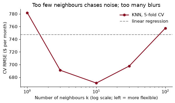
The curve is a U, and it is the bias–variance trade-off you can see. At the left, $k = 1$ copies the rent of the single closest listing, noise and all: low bias, high variance. At the right, $k = 100$ averages over so many listings that real differences are washed out: low variance, high bias. The best value on our grid is $k =$ 10, with a CV RMSE of $671.
Why only “a little”? Each value you try is another chance to fit noise in the cross-validation folds. Five values of one hyperparameter is fine. Five hundred combinations of six hyperparameters, chosen to the last dollar, starts to repeat the best-of-twenty problem one level down. Tune the few settings that matter, on a coarse grid, and stop.
At $k = 1$, the training RMSE (predicting the training listings from the model fitted to them) is $242. The cross-validated RMSE is $782. Explain the gap. Why is the training RMSE not exactly zero?
When a training listing is predicted by a 1-nearest-neighbour model fitted on the training data, its nearest neighbour is usually itself, so the prediction is its own rent and the error is zero. The training RMSE measures memory, not prediction. The CV RMSE asks the honest question, how well it does on listings it has not stored, and the answer is: worse than the linear model.
It is not exactly zero because some listings are identical in every feature but have different rents, two 800 square foot one-bedrooms in the same neighbourhood in the same year at different prices. The model can store only one rent per point in feature space, so it gets one of them wrong. That leftover is a small glimpse of the irreducible error: variation in rent that our features cannot explain, however flexible the model.
Everything is now chosen: the features, the preprocessing, the model, and $k =$ 10. Refit that one model on the whole training set and score it, once, on the 12,426 listings we locked away.
final = make_pipeline(make_prep(), KNeighborsRegressor(n_neighbors=best_k)).fit(X_train, y_train)
test_rmse = root_mean_squared_error(y_test, final.predict(X_test))
The test RMSE is $668 a month, close to the cross-validated $671. That agreement is the point of the exercise: cross-validation promised roughly this, and the untouched data delivered it. For a sense of scale, predicting the training median for every test listing would have missed by $1,400. (That number was not used to choose anything; it is there so a reader knows what $668 means.)
Now the hard part: you do not go back. If the test RMSE disappoints, you may learn something and start a new project with a new test set, but you do not tweak this model and test again. The moment you do, the test set is just another validation set, and you no longer have an honest number.
Write one sentence for the housing office that reports the result. Then say what the sentence should not claim.
“For a typical whole unit in the Bay Area, our model’s rent estimate misses the asking rent by about $668 a month (root mean squared error on 12,426 held-out listings); half the time the miss is smaller than $217, and the average absolute miss is $379.”
It should not claim that the model knows what a bedroom is worth, or that it will be this accurate for units unlike the ones in the data. Most listings are from 2011 to 2016, and they are asking rents on Craigslist, not signed leases. A model is as good as its data on the cases its data cover, and no better.
The whole project, from download to the test score, in one place. It runs top to bottom in the course environment.
from pathlib import Path
import numpy as np, pandas as pd
from sklearn.model_selection import train_test_split, KFold, GridSearchCV
from sklearn.compose import ColumnTransformer
from sklearn.pipeline import Pipeline, make_pipeline
from sklearn.impute import SimpleImputer
from sklearn.preprocessing import StandardScaler, OneHotEncoder
from sklearn.neighbors import KNeighborsRegressor
from sklearn.metrics import root_mean_squared_error
SEED = 368

path = Path("../data/rent.csv")                      # download once, then reuse
if not path.exists():
    path.parent.mkdir(exist_ok=True)
    pd.read_csv(URL).to_csv(path, index=False)
rent = pd.read_csv(path)
Clean, choose features, split. The title is deliberately not among the features.
d = (rent.dropna(subset=["beds", "sqft", "county"])
         .query("room_in_apt == 0 and beds <= 5 and 200 <= sqft <= 5000 and 500 <= price <= 15000"))
num, cat = ["sqft", "beds", "baths", "year"], ["county", "nhood"]
X, y = d[num + cat], d["price"]
X_train, X_test, y_train, y_test = train_test_split(X, y, test_size=0.2, random_state=SEED)
The pipeline, and a small grid search: cross-validation over three values of $k$, on the training data only.
prep = ColumnTransformer([
    ("num", make_pipeline(SimpleImputer(strategy="median"), StandardScaler()), num),
    ("cat", OneHotEncoder(handle_unknown="infrequent_if_exist", min_frequency=50), cat)])
pipe = Pipeline([("prep", prep), ("knn", KNeighborsRegressor())])

search = GridSearchCV(pipe, {"knn__n_neighbors": [5, 10, 20]},
                      cv=KFold(5, shuffle=True, random_state=SEED),
                      scoring="neg_root_mean_squared_error", n_jobs=-1)
search.fit(X_train, y_train)
print(search.best_params_, f"CV RMSE ${-search.best_score_:,.0f}")
{'knn__n_neighbors': 10} CV RMSE $671
GridSearchCV refits the best pipeline on all of the training data when it finishes. That refitted model is the one we score, once.
final_rmse = root_mean_squared_error(y_test, search.predict(X_test))
print(f"Test RMSE: ${final_rmse:,.0f} a month on {len(y_test):,} held-out listings")
Test RMSE: $668 a month on 12,426 held-out listings
Tuning on the test set. Checking the test score, changing something, and checking again. Each look spends a little of its honesty, and you cannot get it back. Choose on cross-validation; test once.
Preprocessing before splitting. Filling missing bathrooms with the median of all the data, scaling with the overall mean, or deciding which neighbourhoods are “common” from the full sample. Each lets the test set shape the training inputs. Put every data-dependent step inside the pipeline.
Features you would not have in time. The rent printed in the ad title is the vivid case. Ask of every column: would I know this at the moment I have to predict? A test set cannot rescue you, because the leak is in the test set too.
Reposts on both sides of the split. Landlords repost the same ad. In our data, 19% of test listings have an exact twin (same rent, size, bedrooms, neighbourhood and year) in the training set. A nearest-neighbour model can look such a listing up rather than predict it, which flatters the score. When the same unit, person or firm can appear more than once, split by group (GroupKFold), or remove duplicates first.
A random split when the future is what you predict. A random split lets the model learn from 2016 ads to predict 2012 ones. If the housing office will use the model on next year’s units, train on earlier years and test on later ones, and expect the error to be larger.
Reading the model as an economist reads a regression. “KNN says an extra bedroom in the Mission adds so many dollars” is not something KNN says. It predicts; it does not explain. If you want what a bedroom is worth, you have a $\hat\beta$ problem.
For each, say whether it is a $\hat\beta$ problem or a $\hat y$ problem, and why. (a) Estimating whether a new BART station raised nearby rents. (b) Deciding which restaurants a city’s three health inspectors visit this week. (c) Imputing missing household income in a survey so that a poverty rate can be computed.
A classmate reports a cross-validated $R^2$ of 0.99 for rents using square feet, county and a column called descr_rent, which she extracted from the description text. What has happened, and what would you tell her to do?
Compute the cross-validated mean absolute error of the median baseline, the linear model and KNN with $k = 10$. Do the three models rank in the same order as under RMSE? (Use scoring="neg_mean_absolute_error".)
Remove reposts before splitting: drop rows that duplicate an earlier row on price, sqft, beds, nhood and year. How many listings remain? Re-run the cross-validation for the linear model and KNN with $k = 10$. How much of KNN’s advantage survives?
Make a time split: train on listings from 2015 and earlier and test on 2016 and later, using the linear model. Compare its RMSE on the later years with the cross-validated RMSE from the random split. Why are they different, and which would you show the housing office?
Take the StandardScaler out of the numeric branch of the pipeline and re-run the cross-validation for KNN with $k = 10$. What happens, and why? Does the linear model care?
A landlord reads that your KNN model predicts $3,803 for her 900 square foot two-bedroom in the Mission and asks how much more she would get if she added a bathroom. What do you tell her?
1. (a) $\hat\beta$: it asks what rents would have been without the station, a counterfactual that needs a design such as difference-in-differences. (b) $\hat y$: the city needs the probability that each restaurant has a violation, and sends inspectors to the highest; this is one of Kleinberg et al.’s examples. (c) $\hat y$: the imputed incomes only need to be close to the truth (and unbiased on average, so the poverty rate is right); nobody will read the imputation model’s coefficients.
2. Leakage. A rent that is extracted from the ad’s own text is the rent, written down by the person who set it, exactly like the price in the title. An $R^2$ of 0.99 on a messy economic outcome is itself a warning sign. Drop the column, ask of every remaining feature whether it would exist before the ad is posted, and re-run.
3.
mae = {name: -cross_val_score(m, X_train, y_train, cv=cv, n_jobs=-1,
                              scoring="neg_mean_absolute_error").mean()
       for name, m in {"median": DummyRegressor(strategy="median"), "linear": ols,
                       "KNN k=10": knn10}.items()}
print({k: round(v) for k, v in mae.items()})
{'median': 916, 'linear': 462, 'KNN k=10': 388}
The MAEs are $916, $462 and $388. The ranking is the same as under RMSE: KNN, then linear, then the median. Each MAE is well below the matching RMSE, because the RMSE is pulled up by the big misses on expensive units.
4.
dd = d.drop_duplicates(subset=["price", "sqft", "beds", "nhood", "year"])
Xd_tr, _, yd_tr, _ = train_test_split(dd[num + cat], dd["price"], test_size=0.2, random_state=SEED)
dedup = {name: cv_rmse(m, Xd_tr, yd_tr).mean() for name, m in {"linear": ols, "KNN k=10": knn10}.items()}
print(len(dd), {k: round(v) for k, v in dedup.items()})
54176 {'linear': 767, 'KNN k=10': 706}
54,176 listings remain (7,953 were reposts). The linear model’s CV RMSE moves to $767 and KNN’s to $706. KNN’s advantage shrinks from $76 to $61: part of it was looking up reposts, but most of it is real.
5.
early, late = d[d["year"] <= 2015], d[d["year"] >= 2016]
ols_time = make_pipeline(make_prep(), LinearRegression()).fit(early[num + cat], early["price"])
rmse_late = root_mean_squared_error(late["price"], ols_time.predict(late[num + cat]))
print(len(early), len(late), round(rmse_late))
45932 16197 802
Trained on 45,932 listings up to 2015, the linear model misses the 16,197 listings from 2016 on by $802, against $747 under the random split. The time split is harder for two reasons: Bay Area rents rose quickly, and year enters linearly, so the model must extrapolate a trend to years it has never seen; and the mix of listings changes over time. Show the housing office the time-split number. It is the honest estimate of how the model will do on the units it will actually be asked about, which are always in the future.
6.
prep_raw = ColumnTransformer([
    ("num", SimpleImputer(strategy="median"), num),
    ("cat", OneHotEncoder(handle_unknown="infrequent_if_exist", min_frequency=50), cat)])
knn_raw = cv_rmse(make_pipeline(prep_raw, KNeighborsRegressor(n_neighbors=10))).mean()
ols_raw = cv_rmse(make_pipeline(prep_raw, LinearRegression())).mean()
print(round(knn_raw), round(ols_raw))
909 748
Without scaling, KNN’s CV RMSE rises from $671 to $909. Distances are now dominated by square feet, which varies by hundreds, and by year, which varies by up to 17. A one-bedroom and a three-bedroom of the same size look like neighbours, and so do two flats in different counties, since a neighbourhood dummy can only differ by 1. The linear model barely notices ($748 against $747): rescaling a feature just rescales its coefficient and leaves the predictions where they were.
7. That the model cannot tell her. It predicts rents for flats like hers by finding similar listings; it was never built to say what changing her flat would do. Flats with two bathrooms differ from flats with one in many ways besides the bathroom (they are bigger, newer, in different buildings). If you force an answer, by changing baths to 2 and predicting again, you will get a number, and it will mix the bathroom with everything that comes with bathrooms. Her question is a $\hat\beta$ problem.
The distinction between $\hat y$ and $\hat\beta$ runs through the rest of the book. These papers make the case for prediction in economics, and say where it stops.
Mullainathan, S. & Spiess, J. (2017). “Machine Learning: An Applied Econometric Approach.” Journal of Economic Perspectives 31(2): 87–106. doi.org/10.1257/jep.31.2.87
The best short introduction to machine learning for economists. The authors predict house values from housing characteristics, compare regression with several machine-learning methods on held-out data, and show that the flexible methods predict better. They then show that a method like the LASSO picks quite different variables in different random subsamples while predicting about equally well, which is their warning against reading the fitted model as the truth about which variables matter.
Think about: the rent model of this chapter could set a housing voucher. Name one decision for which its $\hat y$ is enough, and one (a new zoning rule, a rent subsidy) for which you would need a $\hat\beta$, and explain why the model cannot give you the second.
Kleinberg, J., Ludwig, J., Mullainathan, S. & Obermeyer, Z. (2015). “Prediction Policy Problems.” American Economic Review 105(5): 491–495. doi.org/10.1257/aer.p20151023
Some policy decisions turn on a causal effect and some turn on a prediction. If you are deciding whether to carry an umbrella, you need to predict rain, not to know what causes it. The authors’ example is joint-replacement surgery for elderly patients: the operation pays off only for patients who will live long enough to benefit, so predicting who will die soon can identify surgeries that are likely to be wasted. They argue that many such prediction problems in policy have been neglected.
Think about: if a city began setting vouchers from a rent model, landlords would learn what the model rewards. How could that feedback break the prediction, and why does this make “the world does not respond to my $\hat y$” an assumption worth stating?
Einav, L. & Levin, J. (2014). “Economics in the age of big data.” Science 346(6210). doi.org/10.1126/science.1243089
A short overview of how large private and administrative data sets, from tax records to online transactions, are changing what economists can measure and predict. The authors describe new opportunities in measurement and prediction, the difficulty of turning large data into causal answers, and the problems of access when the most valuable data belong to firms and governments.
Think about: the Craigslist listings in this chapter are a big data set of this kind. Which flats never appear in it (rented by word of mouth, rent-controlled units, luxury buildings with their own websites), and how might that change what the model’s “typical” rent means for a housing office?
Reading. Géron, ch. 1–2, for the landscape of machine learning and a longer project built step by step. ISLP (James, Witten, Hastie, Tibshirani & Taylor 2023), ch. 2 and 5, for the statistics of the bias–variance trade-off and cross-validation. Mullainathan & Spiess (2017), “Machine Learning: An Applied Econometric Approach”, Journal of Economic Perspectives 31(2), for why $\hat y$ is not $\hat\beta$.