The question: a housing office has to set a voucher for a flat nobody has advertised yet. What rent should it expect, in dollars, and how wide a range should it be ready for?
You have met ordinary least squares as an estimator. In econometrics the point of a regression is the coefficient, and the questions you ask of it are about the coefficient: is it unbiased, is it consistent, what is its standard error, have I left out a variable that is correlated with both $x$ and $y$?
In this chapter the same machine does a different job. OLS is a predictor: a rule that takes the features of a flat and returns a guess of its rent. The questions change. Nobody asks whether the coefficient on square footage is causal. We ask how far off the guesses are on flats the model has never seen, and we answer with the test RMSE from Chapter 9.
Here is the model I will build on for most of the chapter. It is a regression of log rent on log square footage, with dummies for the number of bedrooms, the county and the year, fitted to the 49,703 training listings from Chapter 9 (the same cleaning, the same split):
fit = smf.ols("log_price ~ np.log(sqft) + C(beds) + C(county) + C(year)", data=train).fit()
Its test RMSE is 0.252 log points, so a typical miss is roughly 25% of the rent. The training RMSE is 0.250. The two are almost identical, which is what you expect from a model with 33 coefficients and tens of thousands of rows: there is not enough flexibility to memorise anything. Why logs, and how to get back to dollars, is a section of its own below.
The coefficient on log square footage is 0.59. Read as an elasticity, a flat that is 10% bigger rents for about 6% more. As a predictor, that is all it needs to be: a weight that, combined with the others, makes good guesses.
Why is OLS a sensible predictor even when the “true” model is surely not a straight line in these variables? Because of what OLS does: it picks the coefficients that make the squared errors in the training data as small as possible. If the world is not linear, OLS still gives the best linear approximation to it, in the sense of the smallest average squared error. That is exactly the loss we chose in Chapter 9. You do not need to believe the model to use it; you need it to predict well, and you check that on test data.
An estimator is judged by whether $\hat\beta$ is close to $\beta$. A predictor is judged by whether $\hat y$ is close to $y$, on data it has not seen. Same arithmetic, different exam.
A colleague points out that the rent model leaves out the age of the building, the view, and whether there is parking. “Your coefficient on size is biased,” she says. “Bigger flats are in newer buildings.” Is she right, and should the housing office care?
She is right about the coefficient. Bigger flats differ from smaller ones in many ways that also raise rent, so 0.59 mixes the value of space with the value of everything that comes with space. As an estimate of what an extra square foot is worth, holding the flat otherwise fixed, it is biased.
For the housing office it barely matters. The office wants a good guess of the rent of a flat drawn from the same market. If bigger flats tend to come with parking, the size coefficient quietly absorbs some of the value of parking, and the prediction for a big flat is better for it, not worse. Omitted variables make predictions noisier (the variation they would explain ends up in the error), but they do not bias them, as long as the relationship between what is in the model and what is left out stays the same.
That last clause is the catch. If the city starts building large flats without parking, the relationship changes and the predictions go wrong, and nothing in the test RMSE, computed on old listings, would have warned you. Prediction models assume that tomorrow looks like the training data.
How does the computer find the OLS coefficients? For linear regression there is a formula, the normal equation:
\[\hat\beta = (X'X)^{-1}X'y\]where $X$ is the table of features, one row per flat and one column per feature (plus a column of ones for the intercept), and $y$ is the column of log rents.
I do not want you to memorise the matrix algebra. I want you to be able to say what it does, in words:
In numpy it is two lines. patsy turns the formula into the matrix $X$, exactly as statsmodels does behind the scenes:
yv, Xd = patsy.dmatrices("log_price ~ np.log(sqft) + C(beds) + C(county) + C(year)", train)
beta_hat = np.linalg.solve(Xd.T @ Xd, Xd.T @ yv)
The 33 coefficients agree with statsmodels to within 6e-11, which is rounding error.
The normal equation is exact and, for a problem this size, instant. Its weakness is cost as the number of features grows. Computing it means working with $X’X$, a square table with one row and one column per feature, and the work of solving it grows roughly with the cube of the number of features. Double the rows and the job takes about twice as long. Double the features and it takes about eight times as long. With 33 columns nobody notices. With the hundred thousand word counts of a text regression (Chapter 19), or data too big to fit in memory at once, you need another way. That way is gradient descent.
Three hypothetical flats have (centred) log sizes $x = -1, 0, 1$ and log rents $y = 7.0, 7.5, 8.2$. With one feature and an intercept, and $x$ centred at zero, the normal equation reduces to two familiar formulas. What are they, and what are the coefficients?
When $x$ has mean zero, the intercept and the slope untangle completely, and the normal equation becomes
\[\hat\beta_0 = \bar y, \qquad \hat\beta_1 = \frac{\sum_i x_i y_i}{\sum_i x_i^2}.\]The intercept is the mean log rent, $(7.0 + 7.5 + 8.2)/3 = 7.567$. The slope is $(-7.0 + 0 + 8.2)/(1 + 0 + 1) = 1.2/2 = 0.6$. The top of the slope formula is the “how much does $x$ move with $y$” part; the bottom is the “how much does $x$ move with itself” part. With more features, the bottom becomes the whole table $X’X$, but the idea is the same.
Gradient descent is how almost every model after this chapter is trained, from LASSO in Chapter 11 to the neural networks of Chapter 18. It is worth seeing it once on a problem where we know the right answer.
The idea is to forget the formula and walk downhill. The training MSE is a function of the coefficients: pick some $\beta$, and you get some average squared error. Picture that function as a landscape. For linear regression it is a bowl with a single lowest point, which is the OLS solution. Gradient descent starts somewhere (all zeros will do), works out which direction is downhill, takes a step that way, and repeats.
“Which direction is downhill” is the gradient, the vector of slopes of the MSE with respect to each coefficient. For the MSE of a linear model it is
\[\nabla \text{MSE}(\beta) = \frac{2}{n}X'(X\beta - y).\]Read it from the inside out. $X\beta - y$ is the column of current errors. $X’$ times the errors asks, for each feature, whether the errors are large where that feature is large. If they are, that coefficient is too big and the gradient says so. Each step moves $\beta$ a little against the gradient:
\[\beta \leftarrow \beta - \eta\, \nabla \text{MSE}(\beta),\]where $\eta$ (eta) is the learning rate, the size of the step. It is a hyperparameter, like $k$ in nearest neighbours.
Here it is in numpy, on a small version of the rent model with three standardised features (log size, bedrooms, year) so the numbers are easy to look at:
cols = ["sqft", "beds", "year"]
Z = train[cols].assign(sqft=np.log(train["sqft"]))
Z = ((Z - Z.mean()) / Z.std()).to_numpy()
X3 = np.column_stack([np.ones(len(Z)), Z])          # intercept + 3 standardised features
y3 = train["log_price"].to_numpy()

def batch_gd(eta, steps=200):
    b, path = np.zeros(X3.shape[1]), []
    for _ in range(steps):
        err = X3 @ b - y3
        b = b - eta * 2 / len(y3) * X3.T @ err         # one step downhill
        path.append(np.mean(err ** 2))
    return b, path
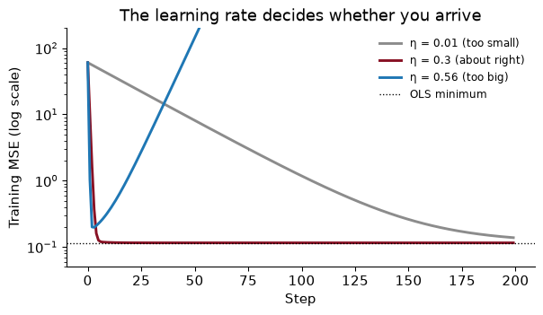
After 200 steps with $\eta = 0.3$, the coefficients agree with the normal equation to within 7e-10. With $\eta = 0.01$ they are still off by up to 0.14. With $\eta =$ 0.56 they never arrive at all:
That picture is the learning-rate trade-off. Too small, and every step is safe but you need thousands of them. Too big, and each step overshoots the bottom of the bowl, lands higher up the other side, and the next step overshoots further: the error explodes. The best learning rate is as large as possible without overshooting.
Standardising the features matters here, as it did for nearest neighbours. If square footage were left in raw units (hundreds to thousands) next to bedrooms (one to five), the bowl would be a long narrow valley: steep across the square-footage direction and nearly flat along the bedrooms direction. Any step size small enough not to overshoot in the steep direction would crawl in the flat one.
Batch gradient descent, the version above, uses every training row to compute each step. With 49,703 rows that is fine; with a billion it is not. Two cheaper versions look at fewer rows per step.
One full pass through the training data is called an epoch. Five epochs of mini-batches of 64 rows is 3,880 small steps, and it lands within 0.011 of the exact coefficients. scikit-learn’s SGDRegressor does the same with more care about the learning rate.
For linear regression on data that fit in memory, none of this beats the normal equation, and LinearRegression does not use it. The point is that gradient descent works for any loss you can take slopes of, with or without a formula, which is why you will see it again in Chapter 11 (as a form of regularisation) and in Chapter 18 (as the only way to train a neural network).
For a linear model, there is a largest learning rate beyond which batch gradient descent explodes. It depends on how steep the bowl is in its steepest direction. For our three-feature model that limit is 0.538. Our “too big” rate was 0.56, only 5% over the limit. Why does such a small excess make the error explode rather than merely slow things down?
Because overshooting compounds. In the steepest direction, a step at the limit lands exactly as far past the bottom as it started, on the other side; it bounces forever without getting closer. A step slightly over the limit lands slightly further away than it started, every time. After one step you are 5% further from the bottom along that direction, after two steps about 10%, and after 200 steps about $1.05^{200} \approx$ 17,293 times as far. That is why the blue line in the figure first drops, as the gentler directions still improve, and then climbs steadily once the one runaway direction takes over. Learning rates fail fast and visibly, which is a mercy: if your training loss is rising, halve $\eta$ before you suspect anything else.
Chapter 9 predicted rent in dollars. This chapter has been predicting log rent. There are three reasons to prefer logs for prices, wages and incomes, and you have met them all in econometrics.
But the housing office pays vouchers in dollars, so at some point we must turn a predicted log rent back into rent. The obvious move is to take the exponential, $e^{\widehat{\log y}}$. It is wrong in a predictable direction.
The reason is that the exponential of an average is not the average of the exponential. The regression predicts the mean of log rent for flats like this one. Exponentiating gives (roughly) the median rent of those flats, and with a right skew the mean rent is above the median. So naive predictions come in too low on average. On the test set the average actual rent is $2,590; the average naive prediction is $2,494.
The fix is due to Duan (1983) and is called the smearing estimator. Multiply every naive prediction by one number, the average of $e^{\text{residual}}$ over the training data:
\[\hat y_{\text{dollars}} = e^{\widehat{\log y}} \times \frac{1}{n}\sum_{i=1}^n e^{\hat\varepsilon_i}\]smear = np.mean(np.exp(fit.resid))
pred_dollars = smear * np.exp(fit.predict(test))
Here the factor is 1.0303, which lifts the average test prediction to $2,569, close to the actual average. Now we can compare the log model with a model fitted directly in dollars, both scored in dollars on the test set:
| Model | Test RMSE, $ a month |
|---|---|
| Rent in dollars on square feet, bedrooms, county, year | $837 |
| Log rent, naive $e^{\hat y}$ | $818 |
| Log rent, with smearing | $809 |
The log model wins even when judged in dollars, and smearing helps a little more. The bigger gain from smearing is not in the RMSE but in the total: a voucher budget built from naive predictions would come up 3.7% short.
(a) The test RMSE of the log model is 0.252. Explain to the housing office what that means in plain words. (b) If the errors were normally distributed with variance $\sigma^2$, the right correction factor would be $e^{\sigma^2/2}$. Compute it from the regression and compare it with the smearing factor.
(a) A miss of 0.25 in log rent is a miss of about 25% of the rent (more exactly, $e^{0.25} - 1 \approx 28\%$ too high, or $1 - e^{-0.25} \approx 22\%$ too low). So “a typical estimate is off by about a quarter of the rent, in one direction or the other”. A percentage is a more honest summary than a dollar figure here, because the size of the miss scales with the rent.
(b) The regression’s residual variance is 0.0624, so $e^{\sigma^2/2} =$ 1.0317, against a smearing factor of 1.0303. They are close but not equal. Smearing does not assume normal errors; it uses the actual residuals, whatever their shape. That is why I use it by default.
The model so far says that a 10% bigger flat rents for about 6% more everywhere in the Bay Area. Is that plausible? Space might be worth more where land is scarce, or less where every flat is already big.
An interaction lets one feature’s slope depend on another. In a formula, np.log(sqft) * C(county) means: the log-size slope, the county dummies, and a separate log-size slope for each county.
fit_int = smf.ols("log_price ~ np.log(sqft) * C(county) + C(beds) + C(year)", data=train).fit()
The implied elasticity of rent with respect to size, county by county:
alameda          0.52
contra costa     0.53
santa cruz       0.56
solano           0.57
sonoma           0.58
santa clara      0.60
san francisco    0.60
san mateo        0.65
marin            0.69
napa             0.70
They range from 0.52 in Alameda to 0.70 in Napa. Those are not small differences in an elasticity. Did they help the prediction? The test RMSE moves from 0.2522 to 0.2514. Barely.
That is a common and useful result. Interactions can be real, and worth knowing about, without mattering much for prediction, because most of the listings are in the counties near the middle of the range and the differences in slope only bite for unusually small or large flats. As in Chapter 9: whether a refinement is worth it is a question about the test error, not about whether the coefficients are significant.
Using the interacted model, how much more does a 1,500 square foot two-bedroom rent than a 1,000 square foot two-bedroom, in 2016, in Alameda and in Napa? Answer in per cent.
The flat is 50% bigger, so the log size rises by $\log 1.5 = 0.405$. Multiply by each county’s elasticity and exponentiate: in Alameda the bigger flat rents for 23% more, in Napa for 33% more. (The bedrooms, year and county intercepts cancel, because they are the same for both flats within a county.) In the additive model the answer would be 27% everywhere.
The economist’s caution again: these are differences between flats that exist, not the effect of building an extension. Large flats in Napa may be large houses with gardens, and the elasticity is carrying the garden.
Size enters the rent model as a log, which is already a curve. For some variables no simple transformation will do, and the classic economic example is age. Wages rise steeply in the first decade of a career and then flatten. A straight line in age misses that shape at both ends.
To see what different methods do, it helps to know the truth, so I simulate it, exactly as in the Lecture 13 notebook: 3,000 CPS-style workers whose log wage depends on schooling, sex and a known age profile, plus noise. Because the data are made up, we know the best possible prediction for every worker, and we know that even that prediction would miss by an RMSE of 0.360 log points, the irreducible error.
The trick that bends a linear regression is to replace age with a few new columns built from age, and run ordinary OLS on those. The model is still linear in its coefficients; only the columns are curved. Two ways to build the columns:
In statsmodels formulas, cr(age, df=6) is a natural spline that uses six columns, and bs(age, df=6) is an ordinary cubic B-spline. The df (degrees of freedom) is the number of columns: more df, more wiggle.
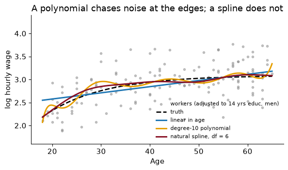
With only 150 workers the differences are stark. The straight line misses the steep early rise. The degree-10 polynomial follows the noise near 18 and 65, where there are few workers to hold it down. The natural spline tracks the truth closely with six columns. Scored on 20,000 fresh simulated workers:
                       coefficients  train RMSE  test RMSE
linear in age                     4       0.392      0.376
quadratic                         5       0.385      0.364
degree-10 polynomial             13       0.374      0.373
natural spline, df = 6            9       0.379      0.365
The degree-10 polynomial has the lowest training RMSE of the four and a worse test RMSE than the spline. You have seen that pattern before, with $k = 1$ in Chapter 9: flexibility that buys a better fit to the training data and pays for it on new data. The spline gets the benefit of bending for little of the cost. Here the humble quadratic does as well, because over ages 18 to 65 the true profile happens to be close to a parabola; the spline did not need to be told that, which is the point of it. Every test RMSE is above the floor of 0.360, as it must be.
scikit-learn has the same tool as a pipeline step, SplineTransformer, which we will use in the In Python section:
from sklearn.preprocessing import SplineTransformer
spline_age = SplineTransformer(n_knots=5, degree=3, extrapolation="linear")
extrapolation="linear" gives the natural-spline behaviour beyond the outer knots.
The simulated workers are aged 18 to 65. A pension office asks for a predicted wage at age 70. What do the degree-10 polynomial and the natural spline (both fitted to the 150 workers) predict, compared with the truth, for a man with 14 years of schooling?
In log points, the truth is 3.08, the natural spline predicts 3.05 and the polynomial 7.81. In dollars an hour (ignoring smearing), that is $22, $21 and $2,471.
The spline continues in a straight line from its last knot, which is a modest and sensible guess. The polynomial’s tenth-power term, which was held in check inside the data, takes over the moment you leave it. Neither model has seen a 70-year-old, and the honest answer to the pension office is that no model fitted to these data can tell them much. But if you must extrapolate, a curve that is linear at the edges is the less dangerous one. (A B-spline from bs() cannot extrapolate at all: it is simply undefined outside the range it was built on, unless you set its bounds by hand.)
How do you know whether a model needs more flexibility, less flexibility, or more data? A learning curve answers that. Train the model on a small sample, then a larger one, then larger still, and at each size record two numbers: the error on the rows it was trained on, and the error on held-out validation rows. Plot both against the size of the training set.
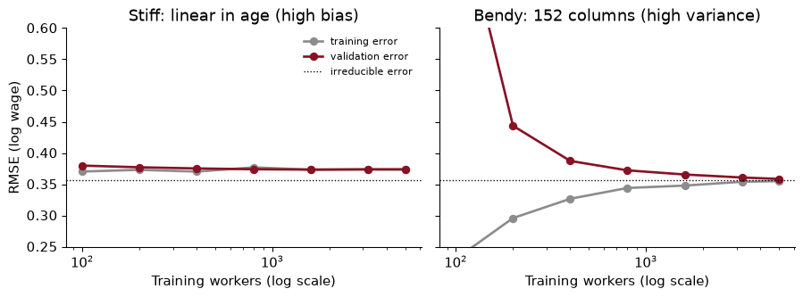
Here are learning curves for two models of the simulated wages. The stiff model is a plain linear regression on age, schooling and sex: three slopes. The bendy model puts a 12-knot spline on age and then adds every square and pairwise product of the resulting columns, 152 columns in all. Each point is the median over 20 random splits, each with 1,000 validation workers.
Read the two shapes.
The stiff model (left) has high bias. Training and validation error are close together even at 100 workers, and from then on they sit side by side on a plateau at about 0.374, above the irreducible error of 0.357 (the RMSE that the true average wage itself scores on the same validation workers). More data does nothing: the model has learned all a straight line can learn. The gap between the plateau and the floor is the price of the wrong shape. The cure is a more flexible model, not a bigger sample.
The bendy model (right) has high variance. With 100 workers its training error is far below the floor (off the bottom of the chart) and its validation error is enormous (0.82, off the top): it is memorising. As the sample grows the gap closes, and by 5,000 workers its validation error is 0.358, below the stiff model’s and close to the floor. More data is exactly what this model needed. If you cannot get more data, the cure is to restrain the model: fewer columns, or the penalties of Chapter 11.
A big gap between training and validation error means variance: get more data or simplify. Two curves that have met at a level you are unhappy with means bias: get a better model or better features.
Draw the learning curve for the log rent model of this chapter, using 5-fold cross-validation on the training listings at sizes from 500 to the full training set. What does it say the housing office should do next: collect more listings, or improve the model?
from sklearn.compose import ColumnTransformer
from sklearn.preprocessing import OneHotEncoder, FunctionTransformer
from sklearn.model_selection import KFold
rent_model = make_pipeline(ColumnTransformer([
    ("size", FunctionTransformer(np.log), ["sqft"]),
    ("cat", OneHotEncoder(handle_unknown="ignore"), ["beds", "county", "year"])]),
    LinearRegression())
n_r, tr_r, va_r = learning_curve(rent_model, train, train["log_price"], cv=KFold(5, shuffle=True, random_state=SEED),
                                 train_sizes=[500, 2_000, 8_000, 20_000, int(0.8 * len(train))],
                                 scoring="neg_root_mean_squared_error")
lc_rent = pd.DataFrame({"train": -tr_r.mean(1), "valid": -va_r.mean(1)}, index=n_r).round(3)
       train  valid
500    0.247  0.257
2000   0.242  0.252
8000   0.251  0.250
20000  0.249  0.250
39762  0.250  0.250
This is the stiff shape. By about 2,000 listings, training and validation error have met at about 0.25, and the next 37,762 listings move the validation error by 0.002. The model is bias-limited. Another 50,000 ads would not help; better features would. Neighbourhood instead of county is the obvious first step (Exercise 4), and the more flexible models of Chapters 14 and 15 are the next. That is a useful thing to know before anyone spends money on data.
A prediction without a range is half an answer. But there are two different ranges, answering two different questions, and mixing them up is one of the most common mistakes in applied work.
Take a 1,000 square foot two-bedroom in San Francisco in 2016. The model’s central prediction is $4,067 a month (in this section I exponentiate without smearing, to keep the two intervals on the same footing).
statsmodels gives both; the confidence interval is mean_ci_lower and mean_ci_upper, the prediction interval obs_ci_lower and obs_ci_upper:
fit.get_prediction(x0).summary_frame(alpha=0.05)
The difference in width is not a detail. The confidence interval shrinks towards zero as the sample grows: with a million listings we would know the average rent of such flats almost exactly. The prediction interval does not shrink below the noise. No amount of data tells you whether this flat has a view.
Are the prediction intervals honest? Check them the way Chapter 8 checked confidence intervals, by coverage: the share of test listings whose actual log rent falls inside their own 95% interval. Overall it is 95.1%, almost exactly right. By county it runs from 90.4% in San Francisco to 98.6% in Solano. The interval uses one noise level for every flat, and rents in San Francisco are harder to predict than elsewhere, so the interval is too narrow there and too wide where rents are steadier.
Two people ask the housing office about 1,000 square foot two-bedrooms in San Francisco. A tenant wants to know what she should expect to pay for one. The office’s budget officer wants to know what 3,000 such vouchers will cost in total. Which interval does each need?
The tenant needs the prediction interval, $2,493 to $6,636. She will rent one flat, with its own luck. Telling her $4,036 to $4,098 would badly overstate how sure anyone can be.
The budget officer is closer to the confidence interval. Over 3,000 flats the individual lucks largely average out (some flats are dearer than predicted, some cheaper), and what remains is uncertainty about the average. Even so, I would give her the average in dollars, which means smearing, since a sum of exponentiated log predictions is too low for exactly the reason the earlier section described. And the confidence interval assumes that these 3,000 flats are like the listings in the data, which is the assumption to check first.
The whole chapter’s model in one runnable place: a log rent model with splines in size and year, neighbourhood dummies, smearing back to dollars, and a test score in dollars.
from pathlib import Path
import numpy as np, pandas as pd
from sklearn.model_selection import train_test_split, KFold, cross_val_score
from sklearn.compose import ColumnTransformer
from sklearn.pipeline import make_pipeline
from sklearn.preprocessing import SplineTransformer, OneHotEncoder, FunctionTransformer
from sklearn.linear_model import LinearRegression
from sklearn.metrics import root_mean_squared_error
SEED = 368

path = Path("../data/rent.csv")                       # download once, then reuse
if not path.exists():
    path.parent.mkdir(exist_ok=True)
    pd.read_csv(URL).to_csv(path, index=False)
rent = pd.read_csv(path)
d = (rent.dropna(subset=["beds", "sqft", "county"])
         .query("room_in_apt == 0 and beds <= 5 and 200 <= sqft <= 5000 and 500 <= price <= 15000"))
X, y = d[["sqft", "beds", "year", "county", "nhood"]], np.log(d["price"])
X_train, X_test, y_train, y_test = train_test_split(X, y, test_size=0.2, random_state=SEED)
Size gets a log and then a spline; year gets a spline; the categories are one-hot encoded, with rare neighbourhoods lumped together as in Chapter 9.
log_spline = make_pipeline(FunctionTransformer(np.log), SplineTransformer(n_knots=6, extrapolation="linear"))
prep = ColumnTransformer([
    ("size", log_spline, ["sqft"]),
    ("year", SplineTransformer(n_knots=5, extrapolation="linear"), ["year"]),
    ("cat", OneHotEncoder(handle_unknown="infrequent_if_exist", min_frequency=50), ["beds", "county", "nhood"])])
model = make_pipeline(prep, LinearRegression())

cv = KFold(5, shuffle=True, random_state=SEED)
cv_log = -cross_val_score(model, X_train, y_train, cv=cv, scoring="neg_root_mean_squared_error")
print(f"CV RMSE: {cv_log.mean():.3f} log points")
CV RMSE: 0.216 log points
Fit once on all the training data, smear, and score once on the test set, in dollars.
model.fit(X_train, y_train)
smear = np.mean(np.exp(y_train - model.predict(X_train)))
pred = smear * np.exp(model.predict(X_test))
print(f"smearing factor {smear:.4f}")
print(f"Test RMSE: ${root_mean_squared_error(np.exp(y_test), pred):,.0f} a month; "
      f"{root_mean_squared_error(y_test, model.predict(X_test)):.3f} log points")
smearing factor 1.0217
Test RMSE: $677 a month; 0.217 log points
The test RMSE in dollars, $677, compares with $809 for the county model earlier in the chapter. For a benchmark, Chapter 9’s nearest-neighbours model with $k = 10$, fitted to the same training listings, misses the same test listings by $668. The linear model is close behind it, and unlike nearest neighbours it can be written down on a page.
Exponentiating log predictions and calling them dollars. $e^{\hat y}$ estimates something close to the median, not the mean, so naive predictions are too low on average: here by 3.7%. For a budget that is real money. Multiply by the smearing factor.
Raw features in gradient descent. Unscaled features turn the bowl into a narrow valley and force a tiny learning rate. Standardise first. And if the training loss goes up as you train, the learning rate is too big; halve it.
Trusting a polynomial at the edges. High-degree polynomials are worst exactly where the data are thinnest, and they are catastrophic outside the data: our degree-10 fit predicts a 70-year-old earns $2,471 an hour. Use a natural spline, and be suspicious of any prediction outside the range of the training data.
Collecting more data for a bias-limited model. If training and validation error have already met, more rows will not move either. Draw the learning curve before you buy data.
Reporting a confidence interval when someone needs a prediction interval. A tenant, a borrower or a benefit claimant is one case, with one case’s luck. The confidence interval for the mean is far too narrow for them.
Reading the predictor as an estimator. The size elasticity of 0.59 is a good predictive weight. It is not the value of an extension, and the county-by-county elasticities are not the value of space in each county. If the decision depends on $\hat\beta$, Chapter 9’s warning applies.
A model of log wages has a test RMSE of 0.40. A model of wages in dollars has a test RMSE of $9.50. Can you tell which is better from these two numbers? What would you compute to compare them?
Write mini-batch gradient descent for the three-feature rent model (log size, bedrooms, year, standardised). Try batch sizes of 1, 64 and 4,096 with a learning rate of 0.01 for two epochs. How far is each from the normal-equation coefficients, and how many updates did each take?
Smearing uses one factor for every flat. Compute the smearing factor separately for each county from the training residuals of the log model, and compare the average predicted rent (naive, single-factor smearing, county smearing) with the average actual rent in each county on the test set. Where does a single factor do worst?
Replace C(county) with neighbourhood dummies in the log model (lumping neighbourhoods with fewer than 50 training listings into “other”, using training counts only). How much does the test RMSE fall? Redraw the learning curve: is the model still bias-limited?
Without computing anything: if the training set were ten times as large, what would happen to the width of the confidence interval and of the prediction interval for the San Francisco flat? Why?
Refit the log model with heteroskedasticity-robust standard errors (cov_type="HC1") and recompute the coverage of the 95% prediction intervals by county. Did it fix the problem in San Francisco? Explain why or why not.
A landlord in Napa reads that the size elasticity there is 0.70 and concludes that a 20% extension will raise her rent by about 14%. What would you tell her?
1. No. The first is in log points, the second in dollars, so they are not in the same units. Put them on the same scale: convert the log model’s predictions to dollars (with smearing) and compute its RMSE in dollars on the same test set, or take logs of the dollar model’s predictions (where positive) and compute its RMSE in log points. Then decide which scale matches the decision. This chapter compared the rent models in dollars because the vouchers are paid in dollars.
2.
def minibatch(batch, eta=0.01, epochs=2, seed=SEED):
    rng, b, steps = np.random.default_rng(seed), np.zeros(X3.shape[1]), 0
    for _ in range(epochs):
        for idx in np.array_split(rng.permutation(len(y3)), max(len(y3) // batch, 1)):
            b = b - eta * 2 / len(idx) * X3[idx].T @ (X3[idx] @ b - y3[idx])
            steps += 1
    return np.abs(b - b_exact).max(), steps
mb = pd.DataFrame({bs: minibatch(bs) for bs in [1, 64, 4096]}, index=["max gap", "updates"]).T
print(mb.to_string(formatters={"max gap": "{:.4f}".format, "updates": "{:,.0f}".format}))
     max gap updates
1     0.0516  99,406
64    0.0059   1,552
4096  4.7727      24
With batches of one row (pure SGD), 99,406 updates get within 0.052: close, but each step is noisy, so it never settles exactly. Batches of 64 take 1,552 updates and land within 0.0059. Batches of 4,096 take only 24 updates, which at this learning rate is not enough to reach the bottom (4.773 off). Larger batches give better steps, but fewer of them per epoch; with large batches you can afford a larger learning rate.
3.
res = train.assign(e=np.exp(fit.resid))
smear_cty = res.groupby("county")["e"].mean()
chk = test.assign(naive=pred_naive, single=pred_smear,
                  by_county=pred_naive * test["county"].map(smear_cty).to_numpy())
gap = chk.groupby("county")[["price", "naive", "single", "by_county"]].mean()
gap_pct = gap[["naive", "single", "by_county"]].div(gap["price"], axis=0) - 1
print(gap_pct.round(3).to_string())
               naive  single  by_county
county
alameda       -0.037  -0.008     -0.008
contra costa  -0.022   0.008      0.009
marin         -0.045  -0.016     -0.009
napa          -0.109  -0.082     -0.077
san francisco -0.051  -0.022     -0.004
san mateo     -0.036  -0.007     -0.015
santa clara   -0.038  -0.009     -0.012
santa cruz     0.000   0.031      0.024
solano        -0.002   0.028      0.014
sonoma        -0.022   0.008     -0.006
Naive predictions are too low, or at best about right, in every county. A single smearing factor fixes most of that. The worst county after smearing is Napa (-8.2%), and a county-specific factor barely helps there (-7.7%). That is not a smearing problem: Napa has only 183 test listings, and a few expensive houses among them can move the average by several per cent. Where county smearing clearly helps is San Francisco, from -2.2% to -0.4%. San Francisco is where the residuals are most spread out, the same heteroskedasticity that made the prediction intervals too narrow there. When the noise differs across groups, smearing by group is a cheap improvement; just check that the groups are big enough for their averages to mean something.
4.
keep = train["nhood"].value_counts().loc[lambda s: s >= 50].index
tr4, te4 = (df_.assign(nh=df_["nhood"].where(df_["nhood"].isin(keep), "other")) for df_ in (train, test))
fit_nh = smf.ols("log_price ~ np.log(sqft) + C(beds) + C(nh) + C(year)", data=tr4).fit()
rmse_nh = rmse(te4["log_price"], fit_nh.predict(te4))
rent_nh = make_pipeline(ColumnTransformer([
    ("size", FunctionTransformer(np.log), ["sqft"]),
    ("cat", OneHotEncoder(handle_unknown="infrequent_if_exist", min_frequency=50), ["beds", "nhood", "year"])]),
    LinearRegression())
n4, tr_4, va_4 = learning_curve(rent_nh, train, train["log_price"], cv=KFold(5, shuffle=True, random_state=SEED),
                                train_sizes=[2_000, 8_000, int(0.8 * len(train))], scoring="neg_root_mean_squared_error")
print(round(rmse_nh, 4), (-tr_4.mean(1)).round(3), (-va_4.mean(1)).round(3))
0.2183 [0.313 0.258 0.216] [0.315 0.254 0.216]
Neighbourhoods cut the test RMSE from 0.252 to 0.218 log points: location within a county matters a great deal. The learning curve is more interesting than before. Training and validation error still meet at every size, so there is no sign of variance. But the validation error now keeps falling as the data grow, from 0.315 at 2,000 listings to 0.216 at full size. The reason is min_frequency=50: in a small sample most neighbourhoods are too rare to get their own dummy and are lumped into “other”; in a large one they earn their own. More data helps this model, through the features it lets the model use. A learning curve tells you about a model and its features together.
5. The confidence interval would shrink, roughly by a factor of $\sqrt{10} \approx 3.2$, because it measures uncertainty about the coefficients, and that falls with the sample size. The prediction interval would hardly change. Most of its width is the noise in individual rents, which does not depend on how many flats we have seen; only the small part that comes from uncertainty about the coefficients would shrink.
6.
fit_hc = smf.ols(FORMULA, data=train).fit(cov_type="HC1")
pi_hc = fit_hc.get_prediction(test).summary_frame(alpha=0.05)
cov_hc = ((test["log_price"].to_numpy() >= pi_hc["obs_ci_lower"].to_numpy())
          & (test["log_price"].to_numpy() <= pi_hc["obs_ci_upper"].to_numpy()))
cov_hc_cty = pd.Series(cov_hc, index=test.index).groupby(test["county"]).mean()
print(pd.DataFrame({"classical": cov_cty, "HC1": cov_hc_cty}).round(3).to_string())
               classical    HC1
county
alameda            0.943  0.943
contra costa       0.969  0.969
marin              0.943  0.943
napa               0.951  0.951
san francisco      0.904  0.904
san mateo          0.969  0.969
santa clara        0.954  0.954
santa cruz         0.974  0.974
solano             0.986  0.986
sonoma             0.979  0.979
It did not. Not a single listing changed sides: coverage in San Francisco is 90.4% either way. Robust standard errors fix the coefficients’ uncertainty when the noise varies. But the prediction interval is mostly the noise itself, and it still uses one noise level for every flat. To fix it you have to model the noise: estimate how the spread of residuals varies by county (or with the features), or use quantile regression or conformal prediction, which build the interval from held-out errors directly.
7. That the number cannot carry that weight. 0.70 describes how rents differ between bigger and smaller flats that exist in Napa, and bigger flats there differ in many ways besides size: more of them are houses, with gardens and parking. An extension adds square feet and nothing else. The prediction model is useful for pricing a flat like the ones in the data; it is not an estimate of what changing a flat would do. That is a $\hat\beta$ question, and it needs a research design, such as comparing the same units before and after renovations.
A rent regression has a long history in economics under another name. These papers explain what its coefficients mean, why Bay Area rents are so high, and how new data are changing the measurement of cities.
Rosen, S. (1974). “Hedonic Prices and Implicit Markets: Product Differentiation in Pure Competition.” Journal of Political Economy 82(1): 34–55. doi.org/10.1086/260169
The theory behind every regression of a price on product characteristics. Rosen treats a flat (or a car, or a job) as a bundle of attributes and asks what the slope of price with respect to one attribute means. His answer is that the price schedule traces out an equilibrium in which buyers with different tastes are matched with sellers who can supply different bundles. The slope at a point tells you what the marginal buyer there pays for a little more, not what any one household would pay, and not a demand curve.
Think about: the chapter’s size elasticity is a slope of this kind. Is it what a particular tenant would pay for 100 more square feet? What would happen to the slope if a wave of families with children moved into the Bay Area, and why does Rosen’s view make the predictive model and the economic interpretation different things?
Glaeser, E. & Gyourko, J. (2018). “The Economic Implications of Housing Supply.” Journal of Economic Perspectives 32(1): 3–30. doi.org/10.1257/jep.32.1.3
The authors compare house prices with the cost of building, and find that in most of the United States homes sell for about what they cost to build. In a few coastal metropolitan areas, the San Francisco Bay Area among them, prices are far above construction cost. They attribute the gap mainly to restrictions on building, and argue that it keeps workers out of the most productive places, with costs for the whole economy.
Think about: the county effects in the chapter’s model capture how much more a similar flat rents for in San Francisco than elsewhere. What supply-side reasons could make that effect so large, and could the prediction model tell you whether allowing more construction would lower rents? What kind of evidence would?
Glaeser, E. L., Kominers, S. D., Luca, M. & Naik, N. (2018). “Big Data and Big Cities: The Promises and Limitations of Improved Measures of Urban Life.” Economic Inquiry 56(1): 114–137. doi.org/10.1111/ecin.12364
The authors show how online and image data can measure cities in ways surveys cannot: for example, predicting the income of a neighbourhood from Street View images, or tracking local businesses from online reviews. They are equally clear about the limits: the measures are predictions, they can miss places that are poorly covered online, and they do not by themselves answer causal questions.
Think about: suppose you added features built from street images to the rent model. What would the model probably learn from them, and what would go wrong if landlords could see which visible features raise the voucher?
Reading. Géron, ch. 4, for the normal equation, the three flavours of gradient descent, polynomial regression and learning curves. ISLP (James, Witten, Hastie, Tibshirani & Taylor 2023), ch. 3 and ch. 7, for linear regression as prediction and for polynomials, splines and generalised additive models. Duan (1983), “Smearing Estimate: A Nonparametric Retransformation Method”, Journal of the American Statistical Association 78(383), for smearing.