The question: a state agency wants to know what centre-based infant care costs in every county, including the ones nobody surveyed. It has fifty-one facts about each county and a few hundred counties to learn from. Which facts should the prediction use, and how much should it trust each one?
Childcare is one of the largest bills a young family pays, and its price is one of the things that decide whether a mother with an infant goes back to work. That makes county childcare prices a real policy input: for subsidy schedules, for judging whether a state’s market is “affordable”, for studies of maternal labour supply.
Our data are the US Women’s Bureau’s National Database of Childcare Prices, as cleaned by TidyTuesday (2023-05-09): a county-by-year panel from 2008 to 2018. The outcome is mc_infant, the median weekly price of centre-based care for an infant. In 2018 the median county charges $154 a week; the 10th percentile is $108 and the 90th $236. Alongside the prices are 51 county covariates from the American Community Survey: unemployment and labour-force participation by sex and age, poverty rates, median household income and earnings, population and households, race and ethnicity shares, how many households with children have both parents working, and employment shares by occupation.
As in Exercise 16, I keep 2018 and model the log price, for the reasons Chapter 10 gave.
Before modelling, look at what is missing, as Chapter 4 taught. The covariates are almost complete: the worst column is missing for 0.006% of county-years, and the pipeline’s median imputer can handle that. The outcome is another matter. In 2018 the infant price is missing for 25% of counties, and the missingness is not scattered. In 10 states it is missing for every county:
Colorado, District of Columbia, Florida, Georgia, Indiana, Iowa, Louisiana, Montana, Nevada, New Mexico
That is 652 counties. In another 5 states some counties are missing. And the pattern moves around over time: in Florida, the share of counties with a 2018 price is 0%, after 97% in 2017. Prices are missing because a state did not submit its market-rate survey that year, not because some kind of county is hard to price.
What do we do about it?
A colleague suggests filling each missing 2018 price with the same county’s price from 2017 and keeping those rows in the training data. Is that a good idea?
It helps the counties that have a 2017 price, and it is a sensible prediction for them: prices move slowly, so last year’s price is a strong guess. But it does three things you should notice. It cannot help the states that are missing in both years. It makes some training “outcomes” into guesses, which the model then fits as if they were measured, with no noise added for the guessing. And it quietly changes the question, from “what do county characteristics predict?” to “what did this county charge last year?”. If last year’s price is available at prediction time, the clean way to use it is as a feature, in a model whose outcome is always a measured price. Imputing an outcome is almost never the right move; imputing a feature, inside the pipeline, often is.
With 51 covariates and 600 training counties, OLS is on reasonably safe ground. But the agency will not always have 600 counties. A state agency working from its own survey might have 60 or 100. And an analyst who wants the model to bend (Chapter 10) quickly multiplies the columns: all squares and pairwise products of 51 covariates are $51 + 51 \times 52 / 2 =$ 1,377 columns.
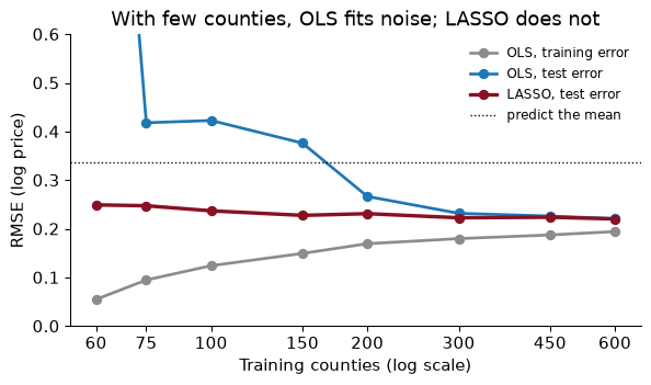
Here is what happens to OLS as the number of training counties shrinks, with all 51 covariates, scored on the same 1,760 test counties:
With 60 counties, OLS fits its training data with an RMSE of 0.055, and misses the test counties by 1.681, worse than predicting the mean for everyone (0.336). With 51 coefficients and 60 counties, it can nearly thread a line through every point, and most of what it learns is noise. The red line is the LASSO, the subject of this chapter: with the same 60 counties it misses by 0.249.
The gap closes as the sample grows. At 600 counties, OLS and LASSO are within 0.001 of each other. But give OLS the 1,377-column wide matrix with the same 600 counties and it fits the training data almost perfectly (RMSE 0.000) and misses the test counties by 1.91 log points, 6 times worse than predicting the mean. With more columns than rows there is no unique least-squares solution at all; the software picks one, and it is garbage.
This is the problem of wide data: many features $p$ relative to rows $n$. It is everywhere in economics: county and tract covariates, survey modules with hundreds of questions, the word counts of Chapter 19, the hundreds of monthly indicators used to nowcast GDP. Chapter 10’s learning curves gave two cures for a model with high variance: more data, or a restrained model. Data are often not for sale. This chapter is about restraint.
(a) Why does the wide matrix have $p + p(p+1)/2$ columns? (b) A colleague adds all cubic terms too (every product of three covariates, including repeats). Roughly how many columns would that be, and what would OLS make of it with 600 counties?
(a) The $p$ original covariates; then every product of two of them, which is $p(p-1)/2$ distinct pairs, plus $p$ squares, for $p(p+1)/2$ in all. With $p = 51$, that is $51 + 1{,}326 = 1{,}377$.
(b) The number of products of three covariates with repeats allowed is $\binom{p+2}{3}$, which for 51 is 23,426. On top of the 1,377, that is over 24,000 columns for 600 counties. OLS would fit the training data exactly, in infinitely many ways, and predict nothing. Flexibility grows much faster than data. That is the whole reason this chapter exists.
OLS chooses the coefficients that make the squared errors as small as possible, and that is all it cares about. If a coefficient of 3.7 on “share of households where both parents work” lowers the training error by a hair, OLS takes it. When there are few rows, many such hairs are noise.
Regularisation (or penalised regression) adds a second goal: keep the coefficients small. Each coefficient now has to earn its keep. It gets to be large only if it improves the fit by more than its size costs. One equation covers both methods we will use:
\[\text{choose } \beta \text{ to minimise} \quad \sum_{i=1}^n (y_i - \hat y_i)^2 \;+\; \lambda \times \text{penalty}(\beta)\]| The LASSO (Tibshirani 1996) measures size as the sum of absolute values, $\sum_j | \beta_j | $. That small change has a large consequence: many coefficients become exactly zero. The LASSO shrinks and selects. |
$\lambda$ (lambda) sets the price of size. At $\lambda = 0$ we are back to OLS. As $\lambda$ grows, coefficients shrink; at a large enough $\lambda$, every coefficient is zero and the model predicts the mean for everyone. $\lambda$ is a hyperparameter, so we will choose it by cross-validation. (scikit-learn calls it alpha, and scales the fit term for the LASSO by $1/(2n)$, so a ridge alpha and a LASSO alpha are not on the same scale. Do not compare them.)
The trade is the bias–variance trade of Chapter 9 in a new form. Shrinking a coefficient towards zero biases it: the true effect of income on prices is not zero, and we are pulling it there. In return, the coefficients wobble much less from sample to sample, so the predictions have lower variance. When the data are few and the features many, the reduction in variance is far larger than the bias, and test error falls.
Why does the absolute value give exact zeros when the square does not? Think about the last little bit of a small coefficient. Under ridge, the penalty on $\beta_j = 0.01$ is $0.0001$, almost nothing, so there is no reason to push it the rest of the way to zero. Under the LASSO the penalty is $0.01$, and it falls by the same amount for every unit of shrinkage, all the way down. If the coefficient is not buying at least that much fit, the LASSO takes it to zero.
Take the simplest case: standardised features that are uncorrelated with each other. Then (with suitable scaling of $\lambda$) the penalised coefficients have simple formulas. If OLS gives $b$, ridge gives $b/(1 + \lambda)$, and the LASSO gives $b - \lambda$ if $b > \lambda$, $b + \lambda$ if $b < -\lambda$, and zero otherwise. Suppose OLS gives hypothetical coefficients of 0.30 on income and 0.04 on the share of service jobs. What do ridge and the LASSO give with $\lambda = 0.05$?
Ridge divides both by 1.05: income becomes $0.30/1.05 = 0.286$ and service jobs $0.04/1.05 = 0.038$. Both shrink by the same proportion, about 5%, and both stay in the model.
| The LASSO subtracts 0.05 from each in absolute value. Income becomes $0.30 - 0.05 = 0.25$. Service jobs has $ | 0.04 | < 0.05$, so it becomes exactly zero: it is out of the model. The LASSO shrinks every coefficient by the same amount, which is a large share of a small coefficient and a small share of a large one, and it drops the ones that cannot pay the toll. |
The penalty adds up the coefficients across features, so it treats a coefficient of 0.1 the same whatever the feature is measured in. But a coefficient’s size depends on its units. Median household income in dollars has a tiny coefficient (a dollar of income is worth almost nothing); the same income in hundreds of thousands of dollars has a coefficient 100,000 times bigger. The penalty would barely notice the first and punish the second hard.
Here is that effect on our data. I standardise every covariate except median household income, leave income in raw units, and fit a LASSO with the same $\lambda$ twice:
| Income measured in | Coefficient on income | Covariates kept |
|---|---|---|
| dollars | 1.31e-05 | 17 |
| hundreds of thousands of dollars | 0.000 | 21 |
Same data, same $\lambda$, and income, which is the single most useful predictor in these data (we will see that shortly), is in the model or out of it depending on a choice of units. Measured in dollars, its coefficient is so small that the penalty is nearly free; measured in units of $100,000, it is too expensive to keep.
The fix is the one from Chapter 9: standardise every feature (subtract its mean, divide by its standard deviation) so that every coefficient is “the change in log price for a one standard deviation change in this covariate”. Then the penalty compares like with like. And the standardisation must be learned from the training data only, which means it goes inside the pipeline: make_pipeline(SimpleImputer(...), StandardScaler(), LassoCV(...)). Each cross-validation fold then standardises using its own training part, and nothing about the held-out fold leaks in.
In the standardised LASSO chosen by cross-validation (coming shortly), the coefficient on median household income is 0.153. The standard deviation of income across the training counties is $14,325. Translate the coefficient into a statement about a $10,000 difference in income.
A one-standard-deviation difference, $14,325, goes with 0.153 higher log price, so $10,000 goes with about 0.153 × 10,000 / 14,325 = 0.107 log points, or roughly 11% higher prices, holding the other selected covariates fixed. To report a coefficient in natural units, divide it by the feature’s standard deviation; to compare the importance of features measured in different units, leave it standardised. And remember that “holding the others fixed” is doing a lot of work in a model whose covariates include four different measures of earnings.
The penalty $\lambda$ is a dial. A coefficient path shows every coefficient at every setting of the dial. Read these from right (huge penalty, everything zero) to left (tiny penalty, close to OLS):
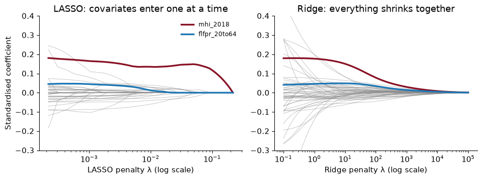
The two pictures tell the difference between the methods better than any formula.
On the LASSO path (left), at the far right every coefficient is zero. Lower the penalty and covariates enter one at a time, each at the point where it becomes worth its price. Median household income (garnet) enters first. Then come one_race_a, memp_n, households, one_race. Female labour-force participation (blue) enters later and stays small. At the far left, with almost no penalty, dozens of covariates are in and some of the paths cross zero and flip sign as their correlated neighbours enter.
On the ridge path (right), every coefficient is nonzero at every penalty; they all shrink smoothly towards zero together as the penalty rises.
Which you want depends on the problem. If you believe a few features carry most of the signal, or you need a short model (a survey that can only ask ten questions), the LASSO’s selection is useful. If you believe many features each matter a little, or the features come in correlated bundles, ridge’s even-handed shrinkage tends to predict better. When in doubt, cross-validate both.
Income is the first covariate the LASSO lets in. Does that make it the most important determinant of childcare prices?
It makes it the single most useful predictor of log price, on its own, among these covariates: when the model can afford only one nonzero coefficient, that is the one that buys the most fit. That is a statement about prediction. It is not a statement that income determines prices. Income is high where wages are high, so it also stands for the wages of childcare workers, the cost of rent for a centre, and the parents’ willingness to pay. Any of those could be doing the work, and the LASSO has no way to tell them apart. It also does not mean the covariates that enter late are unimportant: a covariate that is closely correlated with income has little to add once income is in, however much it matters in the world.
The path shows every possible model; cross-validation picks one. For each $\lambda$ on a grid, run 5-fold cross-validation on the training counties and record the average error; choose the $\lambda$ with the smallest. LassoCV does the whole loop:
lasso_cv = make_pipeline(SimpleImputer(strategy="median"), StandardScaler(),
                         LassoCV(cv=KFold(5, shuffle=True, random_state=368), alphas=60, max_iter=10_000))
lasso_cv.fit(train[covs], train["log_price"])
alphas=60 asks for a grid of 60 values of $\lambda$, spaced evenly on a log scale from the smallest penalty that zeros everything downwards. RidgeCV does the same for ridge, from a grid you supply, using a fast shortcut for leave-one-out cross-validation.
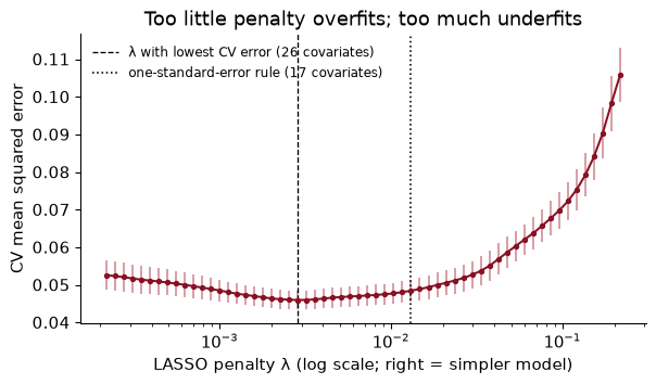
The curve is the U-shape you saw for $k$ in Chapter 9, mirrored. On the right, the penalty is so high that the model is nearly the mean, and error is high (bias). Moving left, useful covariates come in and error falls. Further left, the curve flattens: the extra covariates add little, and with only 600 counties they would eventually add noise. The minimum is at $\lambda =$ 0.0028, which keeps 26 of 51 covariates. Ridge, by the same procedure, picks a penalty of 22.7 and, being ridge, keeps all of them.
Notice how flat the bottom of the curve is. Many values of $\lambda$, and so many different sets of covariates, predict almost equally well. Keep that in mind for the section on instability.
The error bars show that the CV error is itself an estimate, with noise. A popular rule takes the largest $\lambda$ whose CV error is within one standard error of the minimum. What does it choose here, and why would anyone prefer it?
The one-standard-error rule picks $\lambda =$ 0.0131, which keeps 17 covariates instead of 26. Its cross-validated MSE is 0.0485 against 0.0460 at the minimum, a difference smaller than the noise in the estimate itself (one standard error is 0.0025).
Why prefer it? Because the minimum is partly luck: with different folds, it would land somewhere else on the flat bottom. Given two models we cannot tell apart, the simpler one is cheaper to explain, cheaper to collect data for, and less likely to have fitted noise. If the agency must gather every covariate it uses from a separate source, a model with 17 inputs instead of 26 is a real saving for no measurable loss.
The LASSO has a known weakness with correlated features. If two covariates carry nearly the same information (the unemployment rate for everyone aged 16 and over, and for those aged 20 to 64, are correlated at 0.98 across counties), the LASSO tends to keep one and drop the other, and which one is close to arbitrary. Ridge keeps both and splits the weight between them.
The elastic net mixes the two penalties: part sum of absolute values, part sum of squares. scikit-learn’s l1_ratio sets the mix, with 1 meaning pure LASSO and 0 pure ridge. It can still set coefficients to zero, but it tends to keep or drop correlated groups together. Now there are two hyperparameters, $\lambda$ and the mix, and ElasticNetCV cross-validates over both. Here it chooses l1_ratio = 0.9, which is mostly LASSO.
Now every model, chosen on the training counties only, scored once on the 1,760 test counties:
                                test RMSE nonzero coefficients
Predict the training mean           0.336                    0
OLS, 51 covariates                  0.221                   51
Ridge (CV), 51 covariates           0.220                   51
LASSO (CV), 51 covariates           0.220                   26
Elastic net (CV), 51 covariates     0.221                   26
OLS, 1,377 wide columns             1.913                1,377
Ridge (CV), 1,377 wide columns      0.238                1,377
LASSO (CV), 1,377 wide columns      0.220                   84
Four things to read off.
The data have six unemployment rates: overall, female and male, each for ages 16 and over and for ages 20 to 64. Which does the LASSO keep, and which does the elastic net keep?
             LASSO  elastic net
unr_16       0.000        0.000
funr_16      0.011        0.010
munr_16     -0.000       -0.000
unr_20to64   0.000        0.000
funr_20to64  0.000        0.000
munr_20to64  0.043        0.043
The six are correlated with each other at between 0.65 and 0.98. The LASSO keeps 2 of them, and the elastic net keeps 2, with nearly the same weights. With a mix that is 90% LASSO, the elastic net behaves almost exactly like the LASSO here. If you wanted the whole family kept together, you would push l1_ratio towards ridge, and accept the cross-validation’s verdict on whether that predicts better. Note also that the LASSO kept the male 20-to-64 rate and the female 16-plus rate rather than the overall rates. Nobody should read anything into that; see the next section.
The LASSO hands you a list: these 26 covariates matter, the others do not. It is tempting to read that list as a finding. Do not.
To see why, refit the LASSO, with the same $\lambda$, on 30 bootstrap samples of the training counties (600 counties drawn with replacement, as in Chapter 8), and record which covariates are selected each time.
rng = np.random.default_rng(368)
selected = []
for b in range(30):
    idx = rng.choice(len(Xm), len(Xm), replace=True)
    selected.append(Lasso(alpha=lcv.alpha_, max_iter=10_000).fit(Xm[idx], y[idx]).coef_ != 0)
freq = pd.Series(np.mean(selected, axis=0), index=covs)
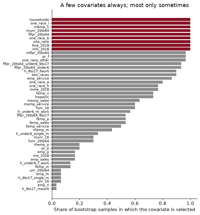
Only 9 covariates are selected in every resample. 38 are selected in some resamples and not others, and only 4 are never selected. The data barely changed (each bootstrap sample is the same 600 counties, reshuffled), and the story about “which variables matter” changed a lot.
The predictions, by contrast, hardly move, because when one covariate drops out, a correlated one picks up its weight. That is the point Mullainathan and Spiess (2017) make about prediction models in general: many different sets of variables predict almost equally well, and the procedure that picks among them is choosing between near-ties. The model is stable where it matters (the $\hat y$) and unstable where people like to look (the list of $\hat\beta$s).
Some of the covariates are nearly the same variable. total_pop and households are correlated at 0.998; one_race and two_races are shares that add up to 100%, so they are correlated at exactly -1. How often does the LASSO pick each of the population twins across the bootstrap samples, and what should you conclude?
Here the LASSO is consistent: households is selected in 100% of the bootstrap samples and total_pop in 0%. That looks like a verdict, households in, population out. It is not. Delete households from the covariates and refit: total_pop steps straight in, with a coefficient of 0.050 (households had 0.078), and the cross-validated RMSE moves from 0.2144 to 0.2160. The two are interchangeable; households happens to edge out population by a sliver of fit, sample after sample. You should conclude nothing about population versus households. If the question “does county size predict childcare prices?” matters, ask it of the group: refit with one twin removed, as here, or use ridge or the elastic net, which share weight across the group.
Here is a sentence a journalist might write after reading our model: “Counties where more women work have more expensive childcare, so policies that raise female employment will push childcare prices up.”
The coefficient behind it is real. Female labour-force participation (ages 20 to 64) is selected, with a standardised coefficient of 0.038: a one-standard-deviation higher participation rate (7.8 percentage points) goes with roughly 4% higher prices, holding the other selected covariates fixed. And still the sentence is wrong, for three reasons.
Causation could run the other way. Where childcare is cheap, more mothers of young children can afford to work, which would make participation higher where prices are lower. Where childcare is expensive, some mothers stay home. The coefficient mixes those effects with any effect of participation on prices, and nothing in the data separates them.
The coefficient carries whatever the covariate stands for. High-participation counties differ in many ways: they are richer (the correlation with median income is 0.54), more urban, with different industries. Drop the four income and earnings covariates from the model and the coefficient on participation rises from 0.038 to 0.067. Its size depends on what else is in the model, because it is partly standing in for income. A LASSO is designed to load weight onto whichever proxy predicts best.
The LASSO biases the coefficient on purpose. Shrinkage pulls every coefficient towards zero; the number is chosen to predict well, not to be close to any true effect.
A LASSO coefficient is a predictive weight, given the other selected covariates. It is not the effect of changing that covariate, and a covariate that was dropped is not one that “doesn’t matter”.
What would you need to answer the journalist’s question? A source of variation in female employment that does not come from childcare prices or from the things that drive both. A randomised experiment is the clean case (Chapter 7); in practice economists use policy changes, such as the introduction of universal pre-kindergarten or expansions of parental leave, in a difference-in-differences design.
A researcher wants the causal effect of a state childcare subsidy on mothers’ employment, and has 51 county covariates to control for. She runs a LASSO of employment on the subsidy dummy and all the covariates, and reports the subsidy coefficient. What is wrong, and is there a right way to use the LASSO here?
Two things are wrong. The penalty shrinks the subsidy coefficient towards zero, so it is biased towards finding no effect, and it might even drop the subsidy from the model entirely. And the LASSO chooses controls that predict employment. A covariate that strongly predicts who got the subsidy but only weakly predicts employment may be dropped, and that is exactly the kind of confounder whose omission biases the estimate.
There is a right way, and it is one of the most useful ideas in modern econometrics: post-double-selection (Belloni, Chernozhukov and Hansen 2014). Run one LASSO of the outcome on the covariates, and a second LASSO of the treatment on the covariates. Take the union of the covariates selected by either, and run ordinary OLS of the outcome on the treatment and that union. The LASSO is used only to choose controls, never to estimate the effect, and the second selection step protects against dropping a confounder. It still needs the usual assumption that, given the controls, the subsidy is as good as random. Machine learning picks the controls; it does not supply the identification.
There is a way to regularise without writing down a penalty at all. Chapter 10 trained a linear model by gradient descent, starting from all coefficients at zero and walking downhill. On a wide matrix, the bottom of the hill is the over-fitted OLS solution. But we do not have to walk all the way there.
Run gradient descent on the 1,377-column wide matrix, using 480 of the training counties to fit and the other 120 as a validation set, and track both errors at every step:
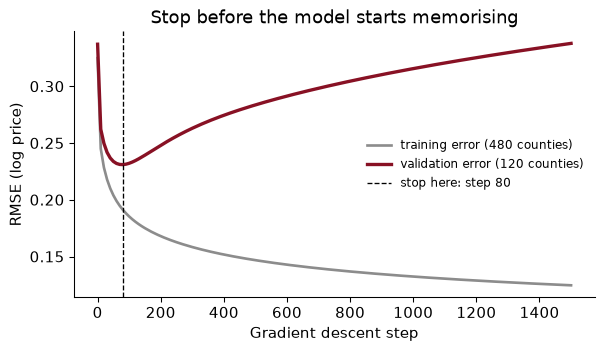
The training error falls at every step, as it must. The validation error falls at first, as the model picks up the main patterns, reaches its minimum at step 80, and then climbs as the model starts fitting the quirks of the 480 counties. Early stopping keeps the coefficients from the best validation step. On the test counties, the early-stopped model scores 0.247; the one that kept going to step 1,500 scores 0.324. Early stopping is not as good here as the LASSO on the same matrix (0.220), but it turns a model that was heading for disaster into a reasonable one with a single decision: when to stop.
Why is this regularisation? Because gradient descent started at zero, and each step lets the coefficients grow a little. Stopping early keeps them small, in much the same way a ridge penalty does: the directions in the data that are strongly supported get learned first, and the weakly supported ones, which is where the noise lives, never get the chance. The number of steps plays the role of $1/\lambda$. It is a hyperparameter, chosen on validation data, never on the test set.
For linear models you would normally just use ridge or the LASSO, which give the same kind of answer more cleanly. Early stopping matters because it works for any model trained by gradient descent, including the boosted trees of Chapter 15 and the neural networks of Chapter 18, where writing down the right penalty is hard and stopping at the right time is easy.
A classmate tracks the test error during gradient descent instead of a validation error, and stops at its minimum. Her test RMSE is a little better than the early-stopped model’s. What has she done wrong?
She has tuned a hyperparameter, the number of steps, on the test set. That is Chapter 9’s cardinal sin in a new costume. The step that minimises test error is the luckiest step for those particular counties, and the test RMSE she reports is the best of many looks, so it is biased downwards. The validation set exists precisely so that the stopping point can be chosen without touching the test set. Then the test set is used once, at the stopping point already chosen.
The whole pipeline, from download to a predicted weekly price in dollars for every county, runnable top to bottom.
from pathlib import Path
import numpy as np, pandas as pd
from sklearn.pipeline import make_pipeline
from sklearn.impute import SimpleImputer
from sklearn.preprocessing import StandardScaler
from sklearn.linear_model import LassoCV
from sklearn.model_selection import KFold
from sklearn.metrics import root_mean_squared_error
SEED = 368
BASE = "https://raw.githubusercontent.com/rfordatascience/tidytuesday/main/data/2023/2023-05-09/"

def load(name):                                        # download once, then reuse
    path = Path(f"../data/{name}.csv")
    if not path.exists():
        path.parent.mkdir(exist_ok=True)
        pd.read_csv(BASE + f"{name}.csv").to_csv(path, index=False)
    return pd.read_csv(path)
cc = load("childcare_costs")
df = cc.merge(load("counties"), on="county_fips_code")
Choose the covariates (never the other price columns), keep 2018, and set aside the counties with no measured price: they are what we want to predict, not what we learn from.
prices = ["mcsa", "mfccsa", "mc_infant", "mc_toddler", "mc_preschool",
          "mfcc_infant", "mfcc_toddler", "mfcc_preschool"]
covs = [c for c in cc.columns if c not in prices + ["county_fips_code", "study_year"]]
d18 = df[df["study_year"] == 2018]
known = d18.dropna(subset=["mc_infant"]).assign(log_price=lambda x: np.log(x["mc_infant"]))
unknown = d18[d18["mc_infant"].isna()]
train = known.sample(600, random_state=SEED)
test = known.drop(train.index)
Impute, standardise and choose $\lambda$, all inside one pipeline fitted on the training counties.
model = make_pipeline(SimpleImputer(strategy="median"), StandardScaler(),
                      LassoCV(cv=KFold(5, shuffle=True, random_state=SEED), alphas=60, max_iter=10_000))
model.fit(train[covs], train["log_price"])
coef = pd.Series(model[-1].coef_, index=covs)
print(f"lambda {model[-1].alpha_:.4f}; {(coef != 0).sum()} of {len(covs)} covariates kept")
print(coef[coef != 0].sort_values(key=abs, ascending=False).head(5).round(3).to_string())
lambda 0.0028; 26 of 51 covariates kept
mhi_2018         0.153
one_race_b      -0.081
households       0.078
h_6to17_fwork   -0.055
fme_2018         0.049
Score once on the test counties, in log points and, with Chapter 10’s smearing, in dollars a week. Then predict the counties with no price.
smear = np.mean(np.exp(train["log_price"] - model.predict(train[covs])))
pred_test = smear * np.exp(model.predict(test[covs]))
print(f"test RMSE {root_mean_squared_error(test['log_price'], model.predict(test[covs])):.3f} log points, "
      f"${root_mean_squared_error(test['mc_infant'], pred_test):.0f} a week")
pred_unknown = smear * np.exp(model.predict(unknown[covs]))
print(f"{len(unknown):,} unsurveyed counties; median predicted price ${np.median(pred_unknown):.0f} a week")
test RMSE 0.220 log points, $36 a week
782 unsurveyed counties; median predicted price $147 a week
Remember what the test RMSE does and does not cover: it is honest for a missing county in a surveyed state, and optimistic for the states with no data at all.
Forgetting to standardise, or standardising outside the pipeline. Without standardisation, the penalty depends on units, and income was in or out of the model depending on whether it was measured in dollars. Standardising the whole data set before splitting leaks the test set’s means into training. Put StandardScaler inside the pipeline.
Leaving the answer in the features. The toddler price, the preschool price and the family-care prices for the same county are all in the data set, and all would predict the infant price superbly. At prediction time, for a county nobody surveyed, none of them exists. Ask of every column, as in Chapter 9: would I have this when I predict?
Reading the selected set as the truth. Only 9 covariates survived every bootstrap resample. The LASSO’s list is one of many near-ties. Never write “the LASSO found that X does not matter”.
Reading a LASSO coefficient as an effect. It is shrunk on purpose, it depends on which correlated neighbours are in the model, and it carries whatever its covariate is a proxy for. For causal questions, use the LASSO to choose controls (double selection), not to estimate.
Choosing λ, or the stopping step, on the test set. Every hyperparameter is chosen by cross-validation or on a validation set. The test set is touched once.
A random split when the real task is a new place. Counties in the same state share regulation, wages and markets, so a random test county has close relatives in training. If the model will be used for states with no data, cross-validate by state (GroupKFold), and expect a larger error.
Explain, without equations, what the LASSO does at $\lambda = 0$ and as $\lambda$ becomes very large. At which end is the bias high, and at which end is the variance high?
Add mc_toddler to the covariates and refit the LASSO pipeline. What happens to the test RMSE, how many covariates does the LASSO keep, and which one has the largest coefficient? Why is this model useless for the agency?
Cross-validate the LASSO pipeline on all 2,360 counties with a measured price in 2018, first with KFold(5, shuffle=True) and then with GroupKFold(5) grouped by state. Compare the two CV RMSEs. Which would you report to an agency that wants prices for the states with no data?
Post-LASSO. Take the covariates selected by LassoCV on the training counties and refit plain OLS on just those. Compare its test RMSE with the LASSO’s. Why might refitting help or hurt?
Add state fixed effects: one-hot encode state_name alongside the scaled covariates (a ColumnTransformer) and refit LassoCV. How much does the test RMSE fall? What does that tell you about where the variation in childcare prices lives, and why is this model of no help for the missing states?
A colleague reports: “The LASSO dropped the poverty rate, so poverty does not affect childcare prices.” Give two reasons this does not follow.
Is the elastic net’s selection more stable than the LASSO’s? Repeat the 30-sample bootstrap with ElasticNet(alpha=..., l1_ratio=0.5) at the elastic net’s cross-validated $\lambda$ for that mix, and compare the number of covariates selected in every resample.
1. At $\lambda = 0$ there is no penalty, so the LASSO is OLS: every covariate is in, and with few counties the coefficients chase noise. That is the high-variance end. As $\lambda$ grows, coefficients shrink and drop out one by one, until at a large enough $\lambda$ all are zero and the model predicts the training mean for every county. That is the high-bias end: the model ignores real information. Cross-validation looks for the setting in between where the sum of the two kinds of error is smallest.
2.
covs_leak = covs + ["mc_toddler"]
leak = make_pipeline(SimpleImputer(strategy="median"), StandardScaler(),
                     LassoCV(cv=KFold(5, shuffle=True, random_state=SEED), alphas=60, max_iter=10_000))
leak.fit(train[covs_leak], train["log_price"])
coef_leak = pd.Series(leak[-1].coef_, index=covs_leak)
leak_rmse = root_mean_squared_error(test["log_price"], leak.predict(test[covs_leak]))
print(round(leak_rmse, 3), (coef_leak != 0).sum(), coef_leak.abs().idxmax())
0.117 24 mc_toddler
The test RMSE collapses from 0.220 to 0.117, the LASSO keeps 24 covariates, and the largest coefficient by far is on mc_toddler. Centres that charge more for infants charge more for toddlers, so the toddler price is nearly the answer. But both prices come from the same market-rate survey: a county with no infant price has no toddler price either. The model answers a question nobody is asking.
3.
from sklearn.model_selection import GroupKFold, cross_val_score
pipe = make_pipeline(SimpleImputer(strategy="median"), StandardScaler(),
                     LassoCV(cv=5, alphas=30, max_iter=10_000))
cv_rand = -cross_val_score(pipe, known[covs], known["log_price"], scoring="neg_root_mean_squared_error",
                           cv=KFold(5, shuffle=True, random_state=SEED)).mean()
cv_state = -cross_val_score(pipe, known[covs], known["log_price"], scoring="neg_root_mean_squared_error",
                            cv=GroupKFold(5), groups=known["state_name"]).mean()
print(round(cv_rand, 3), round(cv_state, 3))
0.217 0.245
With random folds the CV RMSE is 0.217; with folds that hold out whole states it is 0.245, about 13% higher. Holding out a whole state means predicting counties whose regulations, wages and markets the model has never seen, which is exactly the agency’s situation for the dark states. Report the grouped number. (The inner LassoCV(cv=5) still chooses $\lambda$ with random folds; for a fully consistent design you would group those too.)
4.
from sklearn.linear_model import LinearRegression
kept = coef[coef != 0].index.tolist()
post = make_pipeline(SimpleImputer(strategy="median"), StandardScaler(), LinearRegression())
post.fit(train[kept], train["log_price"])
post_rmse = root_mean_squared_error(test["log_price"], post.predict(test[kept]))
lasso_rmse = root_mean_squared_error(test["log_price"], model.predict(test[covs]))
print(len(kept), round(post_rmse, 4), round(lasso_rmse, 4))
26 0.2205 0.2204
Post-LASSO OLS on the 26 selected covariates has a test RMSE of 0.2205, against 0.2204 for the LASSO itself. Refitting removes the shrinkage, which helps when the selected covariates are the real signal and the LASSO had shrunk them too much. It hurts when some selected covariates are noise, because the shrinkage was protecting against them. Here the two are within a hair of each other. Do not report the refitted OLS standard errors as if the covariates had been chosen in advance: they ignore the selection step and are too small.
5.
from sklearn.compose import ColumnTransformer
from sklearn.preprocessing import OneHotEncoder
prep_fe = ColumnTransformer([
    ("num", make_pipeline(SimpleImputer(strategy="median"), StandardScaler()), covs),
    ("state", OneHotEncoder(handle_unknown="ignore", sparse_output=False), ["state_name"])])
fe = make_pipeline(prep_fe, LassoCV(cv=KFold(5, shuffle=True, random_state=SEED), alphas=60, max_iter=10_000))
fe.fit(train[covs + ["state_name"]], train["log_price"])
fe_rmse = root_mean_squared_error(test["log_price"], fe.predict(test[covs + ["state_name"]]))
print(round(fe_rmse, 3), round(lasso_rmse, 3))
0.137 0.22
State dummies cut the test RMSE from 0.220 to 0.137. A large share of the variation in childcare prices is between states: licensing rules, staff-to-child ratios, subsidy rates and wage levels are set or shaped at the state level. For a missing county in a surveyed state, this is the better model. For a state with no data at all there is no dummy to estimate (handle_unknown="ignore" sets them all to zero, which means “an average state”), so it falls back on the covariates alone, and Exercise 3’s grouped CV error is the honest guide.
6. First, the LASSO dropped poverty for prediction, given the other covariates: poverty is strongly correlated with income, unemployment and race shares, which were selected, so it had little extra to offer. That says nothing about its own effect. Second, the selection is unstable: in our bootstrap, pr_f (family poverty) was selected in 97% of resamples and pr_p (individual poverty) in 20%. Whether a poverty measure is “in” depends on which counties happened to be drawn, and on which of two near-identical measures you look at. With slightly different data, the colleague could have written the opposite sentence. And no prediction model, selected or not, estimates what changing poverty would do.
7.
from sklearn.linear_model import ElasticNet, ElasticNetCV
en5 = ElasticNetCV(l1_ratio=0.5, cv=KFold(5, shuffle=True, random_state=SEED), alphas=40, max_iter=10_000).fit(Xm, y)
rng = np.random.default_rng(SEED)
sel_en = []
for b in range(30):
    idx = rng.choice(len(Xm), len(Xm), replace=True)
    sel_en.append(ElasticNet(alpha=en5.alpha_, l1_ratio=0.5, max_iter=10_000).fit(Xm[idx], y[idx]).coef_ != 0)
freq_en = pd.Series(np.mean(sel_en, axis=0), index=covs)
print((freq_en == 1).sum(), ((freq_en > 0) & (freq_en < 1)).sum(), (freq_en == 0).sum())
10 38 3
With a 50/50 mix, 10 covariates are selected in every resample, 38 only sometimes and 3 never, against 9, 38 and 4 for the LASSO. The elastic net is more stable: the ridge part of its penalty keeps correlated covariates in together rather than flipping between them. Either way, the remedy for instability is not a cleverer penalty but a humbler interpretation.
The LASSO arrived in economics with two jobs: choosing controls for causal questions, and predicting with many variables. These papers cover both, plus the market whose prices this chapter predicts.
Belloni, A., Chernozhukov, V. & Hansen, C. (2014). “High-Dimensional Methods and Inference on Structural and Treatment Effects.” Journal of Economic Perspectives 28(2): 29–50. doi.org/10.1257/jep.28.2.29
When you have many possible controls, which ones belong in a regression meant to estimate one causal effect? The authors show that running the LASSO once on the outcome and keeping its survivors can drop a variable that matters because it drives the treatment. Their fix, double selection, runs the LASSO twice, once to predict the outcome and once to predict the treatment, keeps every variable chosen by either, and then estimates the effect by ordinary regression. They apply it to well-known empirical questions and show how it changes conclusions.
Think about: suppose you wanted the effect of a state’s childcare subsidy on county childcare prices, with the fifty-one county facts as possible controls. Why is a variable that predicts which states subsidise (but only weakly predicts prices) dangerous to drop, and what does this tell you about the chapter’s warning not to read LASSO coefficients as effects?
Giannone, D., Lenza, M. & Primiceri, G. E. (2021). “Economic Predictions with Big Data: The Illusion of Sparsity.” Econometrica 89(5): 2409–2437. doi.org/10.3982/ecta17842
The LASSO works best when only a few predictors matter. The authors ask whether economic data really look like that, using a Bayesian model that lets the data choose between a few large effects and many small ones, in data sets from macroeconomics, finance and microeconomics. In most of them the data prefer many small effects. A sparse model can still predict well, but the particular variables it keeps are then one of many near-equivalent choices.
Think about: the chapter found that only a few covariates survived every bootstrap resample. How does this paper explain that instability, and if many county facts each matter a little, what would you tell a state agency that asked which facts “drive” childcare prices?
Herbst, C. M. (2023). “Child Care in the United States: Markets, Policy, and Evidence.” Journal of Policy Analysis and Management 42(1): 255–304. doi.org/10.1002/pam.22436
A survey of the economics of American childcare: why prices are high for families while the workers are among the lowest paid, how regulation such as staff-to-child ratios shapes costs, how public subsidies work, and what the evidence says about their effects on parents’ employment and children’s development. It is the economic background the prices in this chapter’s data lack.
Think about: a prediction model for county prices uses whatever correlates with them. Using Herbst’s account of the market, which features would you expect to matter most (wages, regulation, demand from working parents), and why would a good prediction still not tell you what a new subsidy would do to prices?
Reading. Géron, ch. 4, the section on regularised linear models (ridge, LASSO, elastic net, early stopping). ISLP (James, Witten, Hastie, Tibshirani & Taylor 2023), ch. 6.2, for shrinkage methods and the geometry of why the LASSO gives zeros. Mullainathan & Spiess (2017), “Machine Learning: An Applied Econometric Approach”, Journal of Economic Perspectives 31(2), for why selected variables are not “the” model. Belloni, Chernozhukov & Hansen (2014), “High-Dimensional Methods and Inference on Structural and Treatment Effects”, Journal of Economic Perspectives 28(2), for double selection.