The question: you run a hotel where more than a third of bookings cancel. Should you resell rooms that are already booked, and if so, which ones?
Picture a 200-room hotel, fully booked for tonight. In the data we will use, 119,390 real bookings at two hotels in Portugal between 2015 and 2017, 37% of bookings were cancelled. If tonight is typical, about 74 of your rooms will be empty, and an empty room is a night’s revenue gone.
So you are tempted to resell some rooms. The catch is that a guest who does turn up to a full hotel has to be walked: you pay for a room at a hotel down the road, a taxi, and an apology, and you may lose the customer. Overbook too little and rooms sit empty; overbook too much and you are paying to send guests elsewhere.
Airlines, hotels and car-rental firms all do this, and the field is called revenue management. At its heart is a classification problem. For each booking you want two things, in this order:
They are separate steps, and you can get either one wrong. Most of this chapter is about getting the first right and then not ruining it in the second.
Classification is everywhere in applied economics. A bank deciding on a loan needs the probability of default. A tax authority choosing whom to audit needs the probability of under-reporting. A job-training programme deciding whom to enrol needs the probability of long-term unemployment. Each is a prediction policy problem of the kind we met in Chapter 9, with a label that is yes or no rather than a number.
You know how to regress a 0/1 outcome on features: that is the linear probability model (LPM), and for estimating an average effect near the middle of the data it is often perfectly good. Econometricians use it all the time, and they are right to.
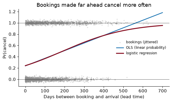
For prediction it has a flaw you can see immediately. A straight line does not know that probabilities stop at 0 and 1. Fit an LPM to the hotel bookings, with all the features we will use later, and 7.1% of the test bookings get a predicted “probability” below zero, while 5.8% get one above one.
That matters more than it sounds, because decisions get made in the tails. The bookings you are thinking of reselling are exactly the ones the model thinks most likely to cancel, and that is where the line overshoots. You cannot multiply a cost by a probability of 1.3.
The LPM predicts $\hat p = -0.08$ for a booking. What does it mean, and what would you do with it?
Taken literally it means nothing: no event has a probability of minus eight per cent. What the model is saying is “this booking looks even less likely to cancel than the bookings that defined the bottom of my line”, and the straight line then runs past zero. You could clip it to 0, and people do. But clipping a prediction after the fact is a sign that the model is the wrong shape. We would rather use one that is built to stay between 0 and 1.
Logistic regression keeps the linear score you know from OLS, $\beta_0 + \beta_1 x_1 + \dots + \beta_k x_k$, and squashes it through an S-shaped curve so that the output is always between 0 and 1:
\[\hat p(x) = \frac{1}{1 + e^{-(\beta_0 + \beta_1 x_1 + \dots + \beta_k x_k)}}\]A very negative score gives $\hat p$ near 0, a very positive score gives $\hat p$ near 1, and a score of zero gives exactly one half. The S-curve is called the sigmoid.
With one feature, lead time, the difference is visible. The line runs above 1 for bookings made far in advance; the S-curve bends to stay below it.
How are the $\beta$s chosen? Not by least squares. Logistic regression uses maximum likelihood: pick the coefficients that make the outcomes we actually saw as probable as possible. A booking that cancelled rewards the model for having given it a high $\hat p$; a booking that showed up rewards a low one. The quantity being minimised has a name you will see in software output, log loss: the average of $-\log(\text{the probability the model gave to what actually happened})$. Its key property is that it punishes confident mistakes brutally. Saying 0.99 for a booking that shows up costs far more than saying 0.6. There is no formula for the answer, as there is for OLS; the computer searches, and because the problem has a single peak, it always finds the same one.
Logistic regression is linear in the log-odds. The odds are $p/(1-p)$: a probability of 0.2 is odds of 1 to 4, or 0.25. Each coefficient says how a one-unit change in $x$ shifts the log-odds, so $e^{\beta}$ is the factor by which the odds are multiplied, the odds ratio.
I say “lightly” because odds ratios are easy to misread. An odds ratio of 2 does not mean “twice as likely”. When the event is rare, odds and probabilities are nearly the same and the shortcut is harmless. When the base rate is 37%, as here, it is not.
Fit a logistic regression of cancellation on the number of special requests a guest made (a cot, a high floor, a late check-in) using the training bookings. The coefficient is -0.722. (a) What is the odds ratio? (b) The model says a booking with no requests cancels with probability 0.458. What does it say for a booking with one request?
(a) The odds ratio is $e$ raised to the coefficient: 0.486. Each extra request multiplies the odds of cancelling by about 0.49, that is, it cuts them by 51%.
(b) Convert to odds, multiply, convert back:
So the probability falls from 46% to 29%. Notice the odds fell by 51% but the probability fell by 36%: odds and probabilities move by different proportions whenever the event is common.
And the economist’s caution: this is a $\hat y$ model, not a $\hat\beta$ one. Guests who ask for a cot are guests who have planned the trip. Nobody believes that the hotel could cut cancellations by encouraging requests.
Before modelling, the question from Chapter 9: would I know this at the moment I have to decide? The hotel decides whether to resell a room before the arrival date. Three columns in the data are recorded later:
reservation_status is “Canceled”, “No-Show” or “Check-Out”, which is the outcome itself, written in words.reservation_status_date is when that status was set.assigned_room_type is the room the guest was actually given at check-in.The first one is not subtle:
is_canceled             0      1
reservation_status
Canceled                0  43017
Check-Out           75166      0
No-Show                 0   1207
Every status lines up with exactly one value of is_canceled. A logistic regression with reservation_status and three innocent features scores 100.0% accuracy on the test set. It is useless, because at decision time the column does not exist yet.
We drop those three, plus agent and company (ID numbers, not quantities) and country, which has more than 170 values; in its place I keep a single dummy, domestic, for guests from Portugal. Then the usual Chapter 9 machinery: a stratified 80/20 split, so that both halves keep the 37% cancellation rate, and a pipeline that fills and scales the numbers and one-hot encodes the categories.
X_train, X_test, y_train, y_test = train_test_split(X, y, test_size=0.2, stratify=y, random_state=368)
logit = make_pipeline(make_prep(), LogisticRegression(max_iter=1000)).fit(X_train, y_train)
p_test = logit.predict_proba(X_test)[:, 1]
predict_proba returns two columns, the probability of each class; column 1 is $\hat p$, the probability of cancelling. The 18 numeric and 8 categorical features become 67 model inputs.
One quick sanity check. The average $\hat p$ on the test set is 0.370, and the actual cancellation rate there is 0.370. A logistic regression with an intercept matches the base rate on average by construction. If yours does not, something is broken.
A classmate shows you a cancellation model with 100.0% test accuracy. She swears she used a proper train/test split. What do you ask her?
What features she used, and when each one becomes known. A test split protects against overfitting; it does nothing against leakage, because the leaked column is in the test set too. An accuracy that high on a messy human outcome (people cancel holidays for all sorts of reasons) is a warning in itself. Here the culprit is reservation_status. In econometric language she controlled for the outcome.
To turn $\hat p$ into a yes/no prediction, the default is to say “cancels” when $\hat p > 0.5$. With that rule, the logistic regression’s accuracy, the share of test bookings it classifies correctly, is 80.8%.
Is that good? Chapter 9’s lesson was to compare everything to a baseline. The laziest classifier predicts “shows up” for every booking. It is right for every booking that did not cancel, so its accuracy is one minus the cancellation rate: 63.0%. The logistic regression is 18 percentage points better. A real gain, but a much less impressive one than “81% accurate” sounds on its own.
A bank’s fraud model is 99.8% accurate. 0.1% of transactions are fraudulent. Is the model any good?
You cannot tell, and there is reason to worry. The rule “nothing is ever fraud” is 99.9% accurate, which beats the model. A fraud model is valuable only if it catches fraud, and accuracy barely registers whether it does: catching every fraud would raise accuracy by at most 0.1 percentage points. With rare events, accuracy is dominated by the easy majority. We need measures that look at the two kinds of mistake separately, which is the next section.
Lay out the four possible outcomes on the 23,878 test bookings, with the 0.5 rule:
| Predict: shows up | Predict: cancels | |
|---|---|---|
| Actually shows up | 13,743 true negatives | 1,290 false positives |
| Actually cancels | 3,286 false negatives | 5,559 true positives |
“Positive” means the model says the event (a cancellation) happens. The diagonal is where the model is right. The two off-diagonal cells are different mistakes, and for the hotel they are very different:
Accuracy adds those two together as if they cost the same. Two measures pull them apart, and they are worth learning as sentences rather than formulas.
Precision: of the bookings we flag as cancellations, what share really cancel? When we resell a room, how often are we right? Here, 5,559 out of 6,849, or 81%.
Recall: of the bookings that really cancel, what share do we flag? Of all the rooms that will sit empty, how many do we catch? Here, 5,559 out of 8,845, or 63%. Recall is also called the true positive rate.
The two pull against each other. Flag more bookings and you catch more cancellations (recall rises) but you also flag more guests who were going to show up (precision usually falls). The threshold is the lever.
Lower the threshold from 0.5 to 0.3. Predict, before computing, what happens to the share of bookings flagged, to recall, and to precision.
| Threshold | Bookings flagged | Recall | Precision |
|---|---|---|---|
| 0.5 | 29% | 63% | 81% |
| 0.3 | 47% | 84% | 67% |
A lower bar flags more bookings. Recall goes up, and it must: every booking flagged at 0.5 is still flagged at 0.3, so we cannot catch fewer cancellations. Precision goes down, because the extra bookings we now flag are the less certain ones, and more of them show up. Precision is not guaranteed to fall, but it usually does.
Which threshold is right depends entirely on what each mistake costs. We will get there; first, a way to see all thresholds at once.
Every threshold gives one confusion matrix, and from each we can read two rates: the true positive rate (recall: the share of cancellations flagged) and the false positive rate (the share of guests who show up that we flag anyway). Plot one against the other for every possible threshold and you have the ROC curve. (The name comes from radar engineers in the Second World War, which is why it is unhelpful.)
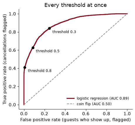
The bottom-left corner is “flag nobody”; the top-right is “flag everybody”. A model that knows nothing traces the diagonal. A perfect model goes straight up the left edge to the top. The black dots are three thresholds; moving the threshold slides you along the curve, it does not move the curve.
The AUC, the area under the curve, summarises it in one number: here 0.889. It has a lovely interpretation. Pick one booking that cancelled and one that did not, at random. The AUC is the probability that the model gives the cancelled one the higher $\hat p$. An AUC of 0.5 is a coin flip; 1 is a perfect ranking.
AUC ignores the threshold. That makes it the right number for comparing how well two models rank bookings, and the wrong number for deciding what to do: no hotel resells a room “at an AUC”.
Verify the interpretation of the AUC by brute force: draw 100,000 random pairs of one cancelled and one kept test booking, and count how often the cancelled one has the higher $\hat p$.
rng = np.random.default_rng(SEED)
p_cancel, p_kept = p_test[y_test.values == 1], p_test[y_test.values == 0]
a, b = rng.choice(p_cancel, 100_000), rng.choice(p_kept, 100_000)
share = (a > b).mean() + 0.5 * (a == b).mean()     # ties count half
The cancelled booking has the higher $\hat p$ in 0.890 of pairs; the AUC is 0.889. Same number, up to the noise from sampling pairs. If you remember one thing about AUC, remember this: it is a statement about ranking pairs, not about any particular decision.
Now the money. Here is what each outcome costs the hotel for one booking:
| Don’t resell | Resell the room | |
|---|---|---|
| Guest shows up | $0 | $300: walk the guest to another hotel |
| Guest cancels | $100: an empty room | $0 |
Walking a guest costs three times as much as an empty room. For a booking with cancellation probability $\hat p$, the expected cost of reselling is $300(1 - \hat p)$, and the expected cost of not reselling is $100\hat p$. Resell when the first is smaller:
\[300\,(1-\hat p) < 100\,\hat p \quad\Longleftrightarrow\quad \hat p > \frac{300}{300 + 100} = 0.75\]In general, act when $\hat p$ exceeds $c_{FP}/(c_{FP} + c_{FN})$, the cost of a false positive over the sum of the two costs. The default 0.5 is what you get if the two mistakes cost the same. Here they do not, so the hotel should resell only when it is quite sure.
The 0.75 assumes $\hat p$ is honest, which we check in the next section. We can also find the threshold directly from data. The rule from Chapter 9 applies: we must not pick it on the test set. So carve a validation set out of the training data, refit on the rest, compute the average cost at every threshold on the validation bookings, and take the cheapest.
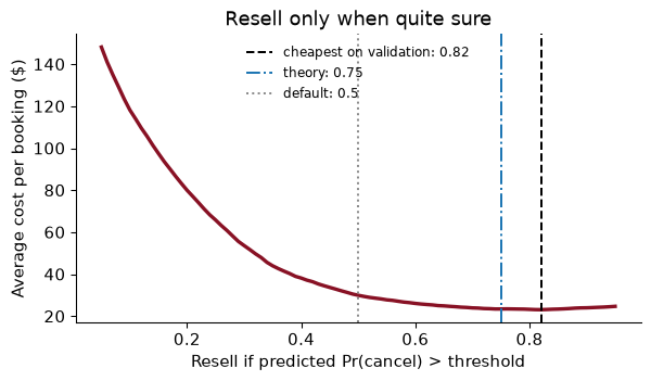
The cheapest threshold on the validation bookings is 0.82, close to the theory’s 0.75. Now, and only now, score it on the test set:
| Rule | Average cost per booking (test) |
|---|---|
| Never resell | $37.04 |
| Resell if $\hat p > 0.5$ | $29.91 |
| Resell if $\hat p > 0.75$ (theory) | $23.77 |
| Resell if $\hat p >$ 0.82 (validation) | $23.31 |
So, should the hotel overbook? Yes, but selectively. Reselling the rooms of bookings with $\hat p >$ 0.82 costs $23.31 a booking, against $37.04 for never reselling and $29.91 for the default threshold. For a full 200-room hotel, moving from 0.5 to the cost-based threshold saves about $1,320 a night. Of the rooms it resells, only 2.5% end up with a guest who has to be walked.
The theory and the data agree to within $0.46 a booking, which is reassuring: it says the probabilities are close to honest. If they had disagreed badly, that would have been the first sign of a calibration problem.
The hotel negotiates a deal with the hotel next door, and walking a guest now costs $150 rather than $300. What is the new theoretical threshold, and what does the validation set say?
The theory gives $150/(150 + 100) = 0.6$. Recomputing the cost curve on the validation bookings with a $150 walk, the cheapest threshold is 0.61. When the expensive mistake gets cheaper, the hotel can afford to be less sure before reselling, so the threshold falls and more rooms are resold. The model did not change at all. The model supplies $\hat p$; the business supplies the threshold.
A cost-based threshold is only as good as the probabilities going into it. A model is calibrated if, among bookings it gives $\hat p \approx 0.3$, about 30% actually cancel. To check, sort the test bookings by $\hat p$, cut them into ten equal groups, and plot the average $\hat p$ in each group against the share that actually cancelled. That is a reliability curve, and an honest model sits on the diagonal.
For our logistic regression, the group whose average $\hat p$ is 0.32 has an actual cancellation rate of 0.33. The full curve is drawn in the next section, next to a model that does much worse.
Calibration matters whenever $\hat p$ is used as a number rather than as a ranking: to set a threshold from costs, to price a non-refundable rate, or to forecast how many rooms will be empty tonight by adding up the $\hat p$s. A model can rank bookings well (high AUC) and still be badly calibrated. Its probabilities can be systematically too extreme, or shifted up or down. One summary is the Brier score, the average of $(\hat p - y)^2$: the mean squared error of the probabilities, lower is better. Here it is 0.127. For scale, always predicting the base rate would score $0.37 \times 0.63 \approx$ 0.233.
If a model is badly calibrated, the fix is to recalibrate it on held-out data: scikit-learn’s CalibratedClassifierCV learns a mapping from the raw scores to honest probabilities. Logistic regression rarely needs it.
Tonight, 200 rooms are booked and the model’s $\hat p$s for those bookings add up to 70.4. How many cancellations do you expect, and why does calibration matter for the answer?
The expected number of cancellations is the sum of the probabilities: about 70. (Each booking contributes its own chance of cancelling, and expectations add.) That is the number a revenue manager uses to decide roughly how many rooms are “spare”. It is right only if the probabilities are calibrated. If the model’s $\hat p$s were all ten points too high, the sum would be twenty rooms too high, the hotel would overbook by twenty, and twenty guests would be walked.
Logistic regression is not the only way to get $\hat p$. Every classifier is trying to approximate the same ideal: if we knew the true probability of cancelling for each kind of booking, we would just predict the likelier class (or apply the cost threshold). That ideal is called the Bayes classifier, and the methods differ in how they approximate it.
There are two broad strategies. Discriminative methods model $\Pr(\text{cancel} \mid x)$ directly. Logistic regression is one. K-nearest neighbours, from Chapter 9, is another: $\hat p$ is the share of cancellations among the $k$ most similar training bookings. Generative methods instead model what each class looks like (what do cancelling bookings look like, and what do kept ones look like?) and then use Bayes’ rule to ask which profile a new booking resembles more, given that 37% of bookings cancel.
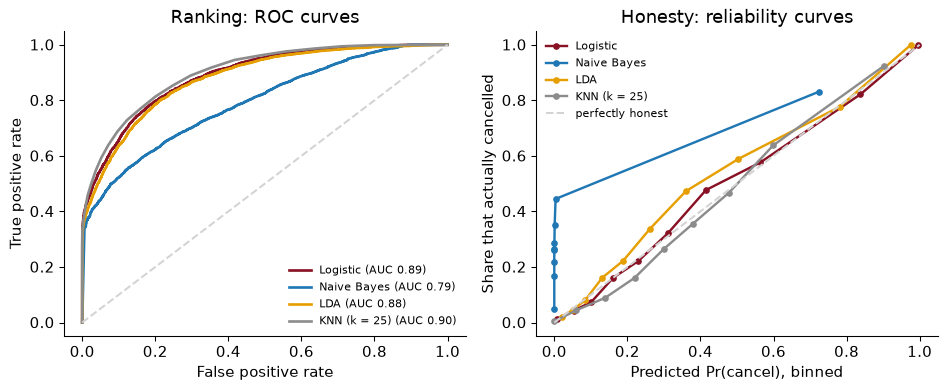
Which is best? There is no general answer: each assumption is right in some worlds and wrong in others, which is why you cross-validate rather than argue. Here they are on the hotel data, each trained on the same 20,000-booking subsample (KNN is slow to predict on large data) and scored on the full test set:
              accuracy  precision  recall    AUC  Brier  flagged
model
Logistic         0.809      0.813   0.628  0.888  0.127    0.286
Naive Bayes      0.758      0.947   0.366  0.792  0.239    0.143
LDA              0.796      0.833   0.562  0.879  0.135    0.250
KNN (k = 25)     0.824      0.808   0.687  0.900  0.122    0.315
Three things to read off.
KNN ranks best. KNN (k = 25) has the highest AUC, 0.900, a little ahead of logistic regression at 0.888. With tens of thousands of bookings, a flexible method that makes no assumption about the shape of the boundary can afford to follow the data.
LDA and logistic regression are close. Both draw straight boundaries; they differ only in how they estimate them. LDA’s AUC is 0.879.
Naive Bayes ranks worst and lies about its probabilities. Its Brier score, 0.239, is worse than predicting the base rate for everyone. Look at its reliability curve: it hugs the edges. Because it treats correlated features (weekend nights and week nights, adults and children) as independent pieces of evidence, it counts the same evidence twice and becomes far too sure of itself, pushing its $\hat p$s towards 0 and 1.
A reasonable conclusion for the hotel: start with logistic regression, which ranks nearly as well as the best, gives honest probabilities without fuss, fits in a second on the full data, and can be explained to a manager. Try a flexible model as a check. Chapters 13 to 15 add support vector machines, trees and boosting, which are often stronger still on data like these.
At the 0.5 threshold, Naive Bayes has the highest precision in the table, 95%, and by far the lowest recall, 37%. Is it the best model for a hotel that cares most about precision?
No. Look at the share of bookings each model flags: Naive Bayes flags 14%, logistic regression 29%. Naive Bayes is simply flagging fewer bookings, only the most obvious ones, so of course a larger share of its flags are right. High precision at one threshold says as much about where the threshold sits as about the model.
The fair comparison is at the same operating point, which is exactly what the ROC curve shows. Logistic regression’s curve lies above Naive Bayes’s everywhere, so if you raised logistic regression’s threshold until it flagged as few bookings as Naive Bayes, it would be at least as precise. Compare models by AUC or by cost at their own best thresholds, never by precision at a single shared threshold.
The model does not use anyone’s name, but it does use where they come from. So ask the question any regulator, journalist or guest would: who bears the cost of the mistakes? Here are the error rates at the cost-based threshold, for guests from Portugal and from abroad:
                    bookings  cancel rate  share resold  walked (of those who show up)  missed (of those who cancel)
guests
international         14,177        0.235         0.009                          0.001                         0.965
domestic (Portugal)    9,701        0.568         0.362                          0.019                         0.377
The difference is stark. Domestic bookings cancel far more often in these data, 57% against 24%, so the model gives them higher $\hat p$s and resells their rooms far more often. The result is that a Portuguese guest who does turn up is walked 1.9% of the time, against 0.08% for an international guest: about 23 times as often. Meanwhile almost every international cancellation goes unnoticed (97% missed).
Is the model “unfair”? It is calibrated and it applies the same threshold to everyone. Dropping the domestic column narrows the gap but does not close it (Exercise 6), because deposit type, lead time and market segment carry some of the same information. (81% of the bookings it resells are on non-refundable rates, which cancel at a startling rate in these data; 97% of non-refundable bookings are by guests from Portugal.) It is doing exactly what we asked. And still, the burden of its mistakes falls almost entirely on one group.
That is not a bug that better engineering will remove. When two groups have different base rates, no model short of a perfect one can be calibrated within each group and give the groups equal false positive rates and equal false negative rates. Kleinberg, Mullainathan and Raghavan (2017) prove it, and Chouldechova (2017) shows the same thing for criminal risk scores. You have to choose which kind of equality you care about, and the choice is about values, not statistics. Fuster, Goldsmith-Pinkham, Ramadorai and Walther (2022) find the same pattern in US mortgage lending, where more flexible machine-learning credit models help some groups of borrowers more than others without ever using group membership directly.
For a hotel the stakes are a ruined evening. For a bank turning down a loan, a court setting bail or a programme choosing whom to train, they are much larger. Whatever the setting, the habit is the same: report error rates by group alongside the overall numbers.
The $300 cost of walking a guest was the hotel’s cost: the other room, the taxi. An international guest who is walked may lose more than a local one (no car, an unfamiliar city, a missed connection). Should the hotel use a different threshold for international guests?
There is a case either way, and writing it down is the point.
For: if walking an international guest really costs the hotel more (worse reviews, lost repeat business), then the cost-based threshold for that group is higher, by the same formula. Here that would mean reselling international rooms even less often, which barely changes anything, since the model hardly ever resells them now.
Against: a group-specific threshold treats guests differently because of where they come from, which is uncomfortable and in some markets unlawful. And the cost matrix only counts the hotel’s own costs. The guest’s lost evening is not in it. If the hotel, or a regulator, decided that a walked guest’s cost counts too, every threshold would rise.
The general lesson: a cost matrix is a statement about whose costs count. Writing it down makes that choice visible, which is better than hiding it inside “we used 0.5”.
The whole analysis in one place, from download to a decision rule, runnable top to bottom.
from pathlib import Path
import numpy as np, pandas as pd
from sklearn.compose import ColumnTransformer
from sklearn.pipeline import make_pipeline
from sklearn.impute import SimpleImputer
from sklearn.preprocessing import StandardScaler, OneHotEncoder
from sklearn.model_selection import train_test_split
from sklearn.linear_model import LogisticRegression
from sklearn.metrics import accuracy_score, precision_score, recall_score, roc_auc_score
SEED = 368

path = Path("../data/hotels.csv")                    # download once, then reuse
if not path.exists():
    path.parent.mkdir(exist_ok=True)
    pd.read_csv(URL).to_csv(path, index=False)
hotels = pd.read_csv(path)
Drop the leaks and the ID-like columns, keep a domestic dummy, split with stratification.
LEAKS = ["reservation_status", "reservation_status_date", "assigned_room_type"]
hotels["domestic"] = (hotels["country"] == "PRT").astype(int)
X = hotels.drop(columns=["is_canceled"] + LEAKS + ["agent", "company", "country"])
y = hotels["is_canceled"]
X_train, X_test, y_train, y_test = train_test_split(X, y, test_size=0.2, stratify=y, random_state=SEED)
num = X.select_dtypes("number").columns.tolist()
cat = X.select_dtypes(exclude="number").columns.tolist()
prep = ColumnTransformer([
    ("num", make_pipeline(SimpleImputer(strategy="median"), StandardScaler()), num),
    ("cat", OneHotEncoder(handle_unknown="ignore", sparse_output=False), cat)])
Choose the threshold on a validation set carved from the training data.
X_fit, X_val, y_fit, y_val = train_test_split(X_train, y_train, test_size=0.25,
                                              stratify=y_train, random_state=SEED)
model = make_pipeline(prep, LogisticRegression(max_iter=1000)).fit(X_fit, y_fit)

def avg_cost(t, p, y_true, walk=300, empty=100):
    resell, y_true = p > t, np.asarray(y_true)
    return (walk * (resell & (y_true == 0)) + empty * (~resell & (y_true == 1))).mean()

grid = np.linspace(0.05, 0.95, 91)
p_val = model.predict_proba(X_val)[:, 1]
t_star = grid[np.argmin([avg_cost(t, p_val, y_val) for t in grid])]
Then score once on the test set.
p = model.predict_proba(X_test)[:, 1]
print(f"AUC {roc_auc_score(y_test, p):.3f} | threshold {t_star:.2f}")
print(f"precision {precision_score(y_test, p > t_star):.3f} | recall {recall_score(y_test, p > t_star):.3f}")
print(f"cost per booking: ${avg_cost(t_star, p, y_test):.2f} vs ${avg_cost(0.5, p, y_test):.2f} at 0.5")
AUC 0.889 | threshold 0.82
precision 0.975 | recall 0.401
cost per booking: $23.31 vs $29.91 at 0.5
Judging by accuracy alone. With a 37% base rate, “nobody cancels” is already 63% accurate; with fraud it is 99.9%. Always put the base rate next to the accuracy, and look at the confusion matrix.
Leaving in a feature recorded after the outcome. reservation_status gives 100% accuracy and is useless. A held-out test set does not catch leakage, because the leak is in the test set too. Ask of every column: would I know this when I decide?
Using 0.5 because it is the default. 0.5 is the right threshold only when both mistakes cost the same, which is almost never. Write down the cost matrix, compute $c_{FP}/(c_{FP} + c_{FN})$, and check it on validation data.
Choosing the threshold on the test set. The threshold is a hyperparameter like any other. Pick it on validation data or by cross-validation, then test once.
Trusting probabilities that have not been checked. A model can rank well and still be miscalibrated, and Naive Bayes on these data is the example. If $\hat p$ feeds a cost calculation, a price or a forecast, draw the reliability curve first.
Reading the coefficients as causal. Non-refundable bookings cancel at 99% in these data, and the model leans on that heavily. That does not mean non-refundable rates cause cancellations; it almost certainly reflects who books them: 97% of non-refundable bookings come through group sales or offline travel agents and tour operators, who block rooms and release the ones they cannot sell. Abolish the rate and those bookings would not turn into reliable guests.
A model gives a booking $\hat p = 0.8$. Which of these is right? (a) This guest will cancel. (b) Among many bookings like this one, about 80% cancel. (c) The model is 80% accurate. (d) The odds of cancelling are 0.8. Explain what is wrong with each of the others.
A credit-card company says a missed fraud costs it $500 and a false alarm (a blocked legitimate purchase and an annoyed customer) costs $10. What threshold on $\hat p$ should it use to block transactions? Is it above or below 0.5, and why does that make sense?
Compute the confusion matrix, precision and recall of the logistic regression at the cost-based threshold, on the test set. Compare them with the 0.5 threshold. Which moved, and in which direction?
Compare the City Hotel and the Resort Hotel: fit the logistic regression on the full training data and report the test AUC separately for each hotel. Is the model better at ranking bookings at one than the other?
Recalibrate Naive Bayes: wrap GaussianNB() in CalibratedClassifierCV(..., method="isotonic", cv=5), fit it on the 20,000-booking subsample, and compare its Brier score and AUC on the test set with plain Naive Bayes. Which number changed, and why did the other barely move?
The fairness table showed that domestic guests who show up are walked far more often. Suppose the hotel drops the domestic column from the model. Predict what happens to the gap, then check it.
Make a time split: train on arrivals in 2015 and 2016 and test on 2017 (column arrival_date_year), dropping arrival_date_year from the features. How does the AUC compare with the random split? What does that tell you about deploying the model?
1. (b). A probability is a statement about many similar cases, not a promise about one. (a) confuses a probability with a decision; the decision comes only after a threshold is chosen. (c) confuses one prediction with the model’s overall accuracy. (d) confuses odds with probability: the odds are $0.8/0.2 = 4$.
2. Block when $\hat p > 10/(10 + 500) \approx 0.02$. That is far below 0.5: a missed fraud is fifty times as costly as a false alarm, so the company should block even when fraud is unlikely. It is the hotel’s logic run the other way. There the expensive mistake was acting (walking a guest), so the bar for acting was high; here the expensive mistake is not acting, so the bar is low.
3.
These use p, from the model fitted in the In Python section on the slightly smaller X_fit, so the 0.5 numbers differ a little from those earlier in the chapter.
from sklearn.metrics import confusion_matrix
for t in [0.5, t_star]:
    print(f"threshold {t:.2f}: precision {precision_score(y_test, p > t):.3f}, "
          f"recall {recall_score(y_test, p > t):.3f}")
    print(confusion_matrix(y_test, p > t))
threshold 0.50: precision 0.812, recall 0.627
[[13752  1281]
 [ 3300  5545]]
threshold 0.82: precision 0.975, recall 0.401
[[14943    90]
 [ 5297  3548]]
Raising the threshold from 0.5 to 0.82 pushes precision up from 81.2% to 97.5% and recall down from 63% to 40%. The hotel resells far fewer rooms, catches fewer cancellations, and almost never walks a guest. That is the right trade when walking is the expensive mistake.
4.
auc_by_hotel = {h: roc_auc_score(y_test[X_test["hotel"] == h], p[(X_test["hotel"] == h).values])
                for h in X_test["hotel"].unique()}
print({h: round(a, 3) for h, a in auc_by_hotel.items()})
{'City Hotel': 0.883, 'Resort Hotel': 0.893}
The test AUC is 0.883 at the City Hotel and 0.893 at the Resort Hotel. The model ranks bookings worse at the City Hotel. Neither number is the AUC of the whole test set, which also gets credit for knowing that city bookings cancel more often than resort ones (42% against 28%).
5.
from sklearn.calibration import CalibratedClassifierCV
from sklearn.naive_bayes import GaussianNB
from sklearn.metrics import brier_score_loss
from sklearn.base import clone
nb_cal = make_pipeline(clone(prep), CalibratedClassifierCV(GaussianNB(), method="isotonic", cv=5))
p_cal = nb_cal.fit(X_small, y_small).predict_proba(X_test)[:, 1]
print(round(brier_score_loss(y_test, p_cal), 3), round(roc_auc_score(y_test, p_cal), 3))
0.162 0.795
The Brier score improves from 0.239 to 0.162. The AUC moves only from 0.792 to 0.795. Recalibration is a monotone relabelling of the scores: it changes what each score means as a probability but (apart from ties and the averaging across folds) not the order of the bookings, and AUC depends only on the order.
6.
X_tr_nd, X_te_nd = X_fit.drop(columns="domestic"), X_test.drop(columns="domestic")   # same data as `model`
prep_nd = ColumnTransformer([
    ("num", make_pipeline(SimpleImputer(strategy="median"), StandardScaler()),
     [c for c in num if c != "domestic"]),
    ("cat", OneHotEncoder(handle_unknown="ignore", sparse_output=False), cat)])
p_nd = make_pipeline(prep_nd, LogisticRegression(max_iter=1000)).fit(X_tr_nd, y_fit).predict_proba(X_te_nd)[:, 1]
walked = pd.Series(p_nd > t_star)[y_test.values == 0].groupby(X_test["domestic"].values[y_test.values == 0]).mean()
cost_nd = avg_cost(t_star, p_nd, y_test)
Without the column, a domestic guest who shows up is walked 0.3% of the time and an international guest 0.11%. The ratio falls from about 23 to about 3: the column was doing a lot of the work, but not all of it. Deposit type, market segment, lead time and the other features are partial proxies for where a guest comes from, so a gap remains.
It is not free. The average cost per booking at the same threshold rises from $23.31 to $23.77, because the model has lost real information. That is the trade-off stated in dollars: the hotel can buy a smaller gap in who gets walked for about $90 a night on 200 rooms. Whether that is worth it is the hotel’s call (or a regulator’s), but now it is a call made with the number in front of you.
7.
tr, te_ = X["arrival_date_year"] <= 2016, X["arrival_date_year"] == 2017
Xt = X.drop(columns="arrival_date_year")
prep_t = ColumnTransformer([
    ("num", make_pipeline(SimpleImputer(strategy="median"), StandardScaler()),
     [c for c in num if c != "arrival_date_year"]),
    ("cat", OneHotEncoder(handle_unknown="ignore", sparse_output=False), cat)])
m_t = make_pipeline(prep_t, LogisticRegression(max_iter=1000)).fit(Xt[tr], y[tr])
auc_time = roc_auc_score(y[te_], m_t.predict_proba(Xt[te_])[:, 1])
Trained on 78,703 bookings from 2015–2016 and tested on 40,687 from 2017, the AUC is 0.851, against 0.889 for the random split. It is lower: a random split lets the model learn from bookings made in the same weeks as the ones it is tested on, which is a luxury a hotel deploying the model never has. The time split is the honest estimate of how the model will do next season.
Classifiers now decide who gets credit and who gets medical care. These two papers ask the chapter’s last question, who bears the cost of the mistakes, with higher stakes than a hotel room.
Fuster, A., Goldsmith-Pinkham, P., Ramadorai, T. & Walther, A. (2022). “Predictably Unequal? The Effects of Machine Learning on Credit Markets.” Journal of Finance 77(1): 5–47. doi.org/10.1111/jofi.13090
The authors compare a logistic-regression model of mortgage default with a more flexible machine-learning model, using US mortgage data. The flexible model predicts better overall, but its gains are not shared equally: white and Asian borrowers are more likely to come out ahead under it, and Black and Hispanic borrowers less likely. Part of the reason is that a flexible model can reconstruct group membership from other variables even when race is not an input.
Think about: in this chapter, dropping the domestic column narrowed the gap between Portuguese and foreign guests but did not close it. Explain why in the language of this paper, and say whether a lender (or a hotel) should be judged by its inputs or by its error rates across groups.
Obermeyer, Z., Powers, B., Vogeli, C. & Mullainathan, S. (2019). “Dissecting racial bias in an algorithm used to manage the health of populations.” Science 366(6464): 447–453. doi.org/10.1126/science.aax2342
A widely used commercial algorithm chose patients for extra care by predicting their future health costs. It predicted costs accurately, for Black and white patients alike. The problem was the target: because less is spent on Black patients with the same health needs, Black patients with a given risk score were sicker than white patients with the same score. Retraining on a direct measure of health instead of cost greatly reduced the disparity.
Think about: the hotel model is well calibrated for is_canceled. Is cancellation the outcome the hotel actually cares about, or a proxy for something else, such as lost revenue or a lost repeat customer? Describe a case in which predicting the label perfectly would still lead to bad decisions.
Reading. Géron, ch. 3, for more on precision–recall trade-offs, multiclass classification and error analysis, and ch. 4 for the logistic regression section. ISLP (James, Witten, Hastie, Tibshirani & Taylor 2023), ch. 4, for logistic regression, LDA, QDA and Naive Bayes side by side. Kleinberg, Mullainathan & Raghavan (2017), “Inherent Trade-Offs in the Fair Determination of Risk Scores”, for the fairness result.