The question: the hotel from Chapter 12 has to decide, booking by booking, whether a room is safe to resell. Does it need a probability for that, or would a well-drawn line between “cancels” and “shows up” do as well or better?
In Chapter 12 we built the hotel’s resale rule in two steps: first a probability $\hat p$ that each booking cancels, then a threshold chosen from what each mistake costs. Logistic regression did the first step well. It ranked bookings well, and its probabilities were honest.
A support vector machine (SVM) takes a different view of the job. It never asks “how likely is this booking to cancel?” It asks a geometric question: where should the line between the two groups go? Every booking is a point in feature space (lead time, daily rate, deposit type, and so on). Cancelled bookings sit mostly in one region, kept bookings mostly in another, and the SVM’s job is to draw the boundary between them as well as it can.
Like logistic regression, a linear SVM gives each booking a score: a weighted sum of its features plus a constant, $f(x) = \beta_0 + \beta_1 x_1 + \dots + \beta_k x_k$. A positive score means “cancels”, a negative one “shows up”, and the decision boundary is where the score is exactly zero. With two features the boundary is a line; with three, a plane; in general it is called a hyperplane, which just means a flat boundary in however many dimensions you have.
The difference from logistic regression lies in how the $\beta$s are chosen, and that difference has consequences. An SVM’s score is not a probability, and nothing pushes it to be one. For many classification problems you never need a probability: a spam filter only needs to know which side of the line an email is on. The hotel is not one of those problems, as we will see at the end of the chapter. But first, the idea.
SVMs were invented by Cortes and Vapnik (1995), and for about fifteen years they were the best off-the-shelf classifier for many tasks, text above all. Deep learning and boosted trees have since overtaken them on most benchmarks. I teach them anyway, for three reasons: the geometry is beautiful and easy to see, the kernel trick is one of the most useful ideas in machine learning, and on medium-sized problems they are still a strong baseline that costs one line of code.
A linear SVM fitted to bookings gives one booking a score of $+2.4$ and another a score of $-0.3$. A colleague says the first is “eight times as likely to cancel”. What can you actually say?
Only two things. The first booking is on the “cancels” side of the boundary and the second is on the “shows up” side, just barely. And the first is further from the boundary, so the model is more confident about it. The ratio of the scores means nothing. A score is a distance-like quantity, measured in units the model chose for its own convenience; it is not a probability and not odds. If you need a probability, you have to build one from the score, which is the last section of this chapter.
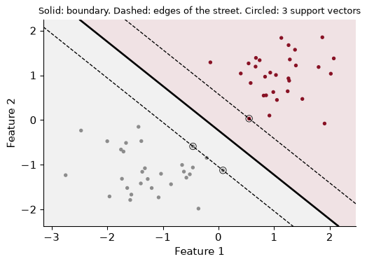
Start with the easiest possible case: two groups that can be separated perfectly by a straight line. The data below are made up, sixty points in two features, so that the geometry is clean. Real bookings come in the next section.
When two groups can be separated, infinitely many lines separate them. You could nudge any separating line a little, or tilt it, and it would still separate. Which one should we pick?
The SVM’s answer: pick the line that leaves the widest street between the two groups. Draw the boundary, then draw two parallel lines on either side of it, as far out as they can go before touching a point. The gap between those two lines is the margin, and the SVM chooses the boundary that makes the margin as wide as possible. This is the maximal margin classifier.
The points sitting exactly on the edges of the street are circled. These are the support vectors, and they give the method its name: they “support” the street the way pillars hold up a roof. Here there are only 3 of them out of 60 points.
Here is the property that makes SVMs unusual. Only the support vectors determine the boundary. Every other point could be moved anywhere, as long as it stays on its own side and outside the street, and the boundary would not move at all. Logistic regression is different: every observation pulls on its coefficients a little.
Why the widest street? The intuition is a safety margin. New bookings will not land exactly where the old ones did. A boundary that scrapes past the training points on one side will misclassify a new point that lands slightly closer; a boundary with room on both sides has a buffer. There is theory behind this (wider margins give tighter bounds on the error on new data), but the buffer is the idea.
Take the point furthest from the boundary and move it twice as far away. Then, instead, move one of the support vectors halfway towards the boundary. Refit the SVM each time. What happens to the boundary?
far = np.argmax(np.abs(hard.decision_function(X_sep)))      # furthest from the boundary
X_far = X_sep.copy(); X_far[far] *= 2
m_far = SVC(kernel="linear", C=1e6).fit(X_far, y_sep)

sv0 = hard.support_[0]                                      # one support vector
X_sv = X_sep.copy(); X_sv[sv0] = X_sv[sv0] - 0.5 * hard.decision_function(X_sep[[sv0]]) * hard.coef_[0] / np.sum(hard.coef_ ** 2)
m_sv = SVC(kernel="linear", C=1e6).fit(X_sv, y_sep)
original coefficients:        [[1.223 1.231]] [0.285]
far point moved further:      [[1.223 1.231]] [0.285]
support vector moved inward:  [[0.834 1.865]] [0.479]
Moving the far point changes nothing, to three decimal places: it was never a support vector, so the SVM never looked at it. Moving a support vector into the street forces the street to narrow and the boundary to shift, because that point now pins one edge. Width goes from 1.15 to 0.98.
That is the strength and the weakness of the maximal margin idea in one picture. It ignores easy cases, which is efficient. But it is hostage to the few cases near the boundary, and in real data those are exactly the ambiguous, noisy ones.
CReal bookings cannot be separated by a line. Take 400 bookings, half of them cancelled and half not (equal numbers make the pictures easier to read), and two features, the (log) lead time and the average daily rate, both standardized. Plenty of cancelled bookings sit right among the kept ones. No street exists that has all the cancellations on one side.
The fix is the soft margin. Let some points sit inside the street, or even on the wrong side of the boundary, but charge a price for each violation, in proportion to how far over the line it is. The SVM now trades off two things: a wide street, and few, small violations.
The price is the hyperparameter C. In scikit-learn:
C: violations are expensive. The SVM narrows the street to keep as many training points as possible on the right side. Fewer support vectors, so the boundary is set by a handful of points near it: low bias, high variance.C: violations are cheap. The street is wide, many points sit inside it, and all of them help set the boundary. A more stable, more averaged boundary: higher bias, lower variance.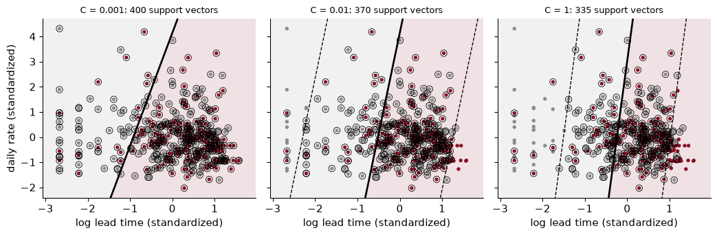
Garnet points cancelled, grey ones did not, and the shaded side is where the SVM predicts a cancellation. The boundary tilts the same way in all three panels: bookings made far ahead cancel more, which we saw in Chapter 12. What changes with C is the width of the street and the number of points that count. At C = 0.001 the street is 16.8 standard deviations wide and 400 of the 400 bookings are support vectors; at C = 1 it narrows to 2.5, with 335 support vectors. Raising C beyond 1 changes almost nothing here: once the street is as narrow as the overlap allows, a higher price for violations cannot buy a cleaner separation that does not exist.
Support vectors are not only the points on the edge of the street. With a soft margin they are every point on the edge, inside the street, or on the wrong side. They are the cases the model finds hard.
A warning about notation, because it trips people up every year. In ISLP, the textbook I recommend for the statistics, $C$ is a budget for violations: bigger $C$ means more violations allowed. In scikit-learn, C is the price of a violation: bigger C means fewer allowed. They point in opposite directions. scikit-learn’s C works like the C in LogisticRegression from Chapter 12: it is the inverse of a ridge penalty, so bigger C means less regularization.
At C = 1, 335 of the 400 bookings, 84%, are support vectors. In the made-up separable data there were 3 out of 60. Explain the difference. What does it tell you about these two features?
A support vector is any point on the edge of the street, inside it, or on the wrong side. When the classes overlap heavily, a large share of points end up in one of those places, because there is no clean gap for them to sit outside. In the made-up data the groups were far apart, so only the few points closest to the gap mattered.
So the count is a diagnostic. Lead time and the daily rate separate cancellations from stays only weakly: a booking’s lead time and price tell you something, but most bookings look ambiguous on these two features alone. That is not a failure of the SVM. The full model, with deposit type, market segment and the rest, does much better, as we will see.
The soft-margin SVM and logistic regression are closer relatives than they look. Both fit a linear score $f(x)$. Both add a ridge penalty on the coefficients (Chapter 11) to keep them from going wild. They differ in exactly one thing: how they charge for each training point.
To compare them, code the outcome as $y = +1$ for a cancellation and $y = -1$ for a stay. Then $y \cdot f(x)$ is positive when the booking is on the correct side of the boundary, and the larger it is, the more safely correct. Call it the booking’s margin. The SVM’s charge is the hinge loss:
\[\text{hinge loss} = \max\big(0,\ 1 - y \cdot f(x)\big)\]In words: a point safely beyond the edge of the street costs nothing at all. Inside the street, or on the wrong side, it costs in proportion to how far it has strayed. Logistic regression’s charge is the log loss from Chapter 12, which in this notation is $\log(1 + e^{-y f(x)})$: it shrinks as a point gets more safely correct, but it never reaches zero.
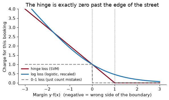
The dashed grey line is what we really care about, the count of mistakes: 1 for a misclassified point, 0 for a correct one. Nobody minimises it directly, because its jump at zero makes it impossible to search over. The hinge and the log loss are both smooth-ish stand-ins for it, and both punish a confident mistake more than a near miss.
The flat part of the hinge is the whole story. A booking that is safely classified contributes nothing to the SVM’s objective, so moving it changes nothing. That is why only support vectors matter. Logistic regression listens to everyone, a little.
In practice, when the classes overlap as much as cancellations and stays do, the two methods draw almost the same line. What really separates them is the output. Logistic regression gives probabilities as a by-product of its loss: log loss is the likelihood, so the fitted $\hat p$s are built to be honest. The hinge loss has no such interpretation. It cares only about which side of the street a point lands on.
Three cancelled bookings ($y = +1$) get scores $f(x)$ of $-0.5$, $0.5$ and $2$. Compute each booking’s hinge loss and log loss. Which booking does each method care about most, and which does the SVM ignore?
The margins $y \cdot f(x)$ are just the scores, since $y = +1$.
| Score | Where it is | Hinge loss | Log loss |
|---|---|---|---|
| −0.5 | wrong side | 1.50 | 0.974 |
| 0.5 | right side, inside the street | 0.50 | 0.474 |
| 2 | safely past the edge | 0.00 | 0.127 |
Both methods charge most for the misclassified booking. The SVM ignores the third booking completely: its hinge loss is exactly zero, so it is not a support vector. Logistic regression still charges it 0.127, a small amount, so it still nudges the coefficients.
So far every boundary has been a straight line. Suppose, though, that the truth is curved. Here is a made-up example that is not far-fetched: bookings made at the last minute cancel often (a business trip that falls through), bookings made very far ahead cancel often (plans change), and bookings in the middle mostly show up. On a single feature, lead time, the cancellations sit at both ends. No single cutoff separates them.
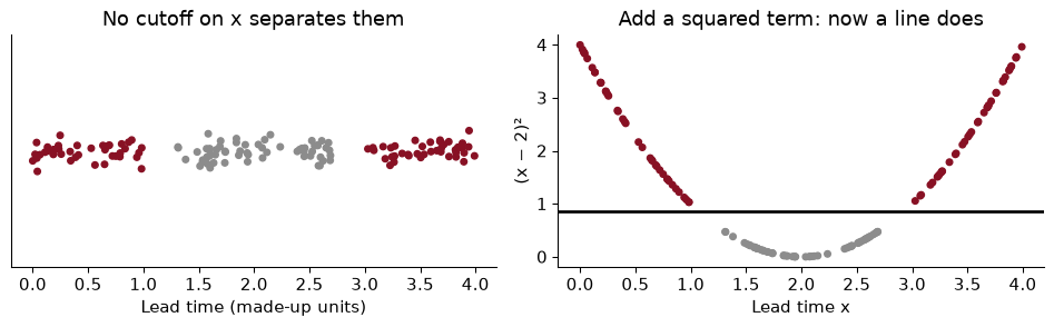
The trick on the right is one you know from econometrics: add a squared term. In the enlarged space, with $x$ and $x^2$ as two features, a straight line separates the groups, and a straight line in the enlarged space is a curve (here, two cutoffs) in the original one. Chapter 10 did the same thing with polynomial regression.
The trouble is scale. With 30 features, all the squares and pairwise interactions come to nearly 500 columns; all the terms up to degree 3 come to several thousand. Building them is slow and the model drowns in them.
Here is the kernel trick. When you work through the mathematics of the SVM, the data turn out to enter the problem only through one quantity: how similar each pair of bookings is. The SVM never needs the features themselves, only a similarity score for every pair. A kernel is a function that computes that similarity, and different kernels correspond to different enlarged feature spaces, without ever building them. You get the curved boundary of a huge feature space at the cost of computing similarities.
Three kernels do almost all the work in practice:
The RBF kernel is 1 when two bookings are identical and falls towards 0 as they move apart. A prediction for a new booking is then a weighted vote of the support vectors, each weighted by how close it is to the new booking. If that sounds like nearest neighbours from Chapter 9, it should: the RBF SVM is a smooth cousin of KNN, in which every support vector votes but near ones count far more. The feature space it corresponds to is infinitely large, which is a fact worth knowing and not worth worrying about.
Back to the 400 bookings and our two features. To judge each boundary honestly, I score it on 3,000 fresh bookings that the SVM never saw.
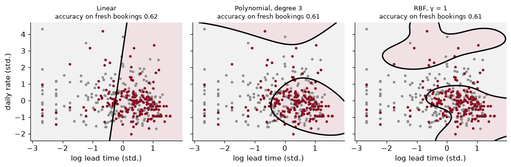
The linear boundary is a straight cut. The polynomial and RBF kernels bend it, carving out a region of long lead times and moderate prices where cancellations concentrate. On fresh bookings (also half cancellations, so guessing scores 0.50) the three are close, 0.61 to 0.62 accuracy, and the straight line is the best of them. Two weak features do not leave much room for any curve to pay off. Curves earn their keep when there are many features whose effects depend on each other, which is the full hotel data later in the chapter.
The RBF kernel has its own hyperparameter, $\gamma$ (“gamma”). It sets how fast similarity falls with distance, and so how local the vote is.
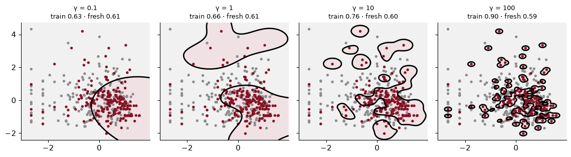
Read the titles left to right. Training accuracy climbs from 0.63 to 0.90 as the boundary gets more flexible. Accuracy on fresh bookings does not follow: it drifts down from 0.61 to 0.59. The picture shows why: at $\gamma$ = 100 the “cancels” region is a scatter of islands around individual training bookings, a map of this sample’s noise.
C and $\gamma$ both control flexibility, so they interact. A large $\gamma$ can be tamed by a small C, and the other way round. Tune them together, which we will do on the full data shortly.
Two bookings, after scaling, differ by 1.0 in log lead time and by 0.5 in daily rate. What is their RBF similarity at $\gamma$ = 0.1, 1 and 10? What does that say about how much one would influence a prediction for the other?
The squared distance is $1.0^2 + 0.5^2 = 1.25$. The similarity is $e^{-\gamma \times 1.25}$:
| $\gamma$ | Similarity |
|---|---|
| 0.1 | 0.882 |
| 1 | 0.287 |
| 10 | 0.000004 |
At $\gamma$ = 0.1 the two bookings are almost interchangeable: each would count nearly fully in the vote for the other. At $\gamma$ = 10 they are strangers: a distance of about one standard deviation is already far enough to cut the influence to almost nothing. Same two bookings, same distance; $\gamma$ alone decides whether they are “neighbours”.
Margins are distances and the RBF kernel is built on distances, so an SVM inherits KNN’s sensitivity to units (Chapter 9, Exercise 6). A feature measured in big numbers dominates the distance and the others barely register.
In the hotel data the problem is severe. Among the numeric features, the standard deviation of lead_time (in days) is 107 and of adr (the daily rate, in euros) 51. Meanwhile domestic, is_repeated_guest and every one-hot dummy can only differ by 1.
From here on I use a training subsample of 10,000 bookings for kernel SVMs, for a reason the section on big data below makes clear. Cross-validated on that subsample, an RBF SVM with default settings has an AUC of 0.900 with the numeric features standardized and 0.697 without. Same data, same model, same hyperparameters. The only difference is the units.
The fix is the same as in Chapter 9: put a StandardScaler inside the pipeline, so that the scaling is learned on the training folds only. The one-hot dummies are left at 0/1, which is the usual compromise.
Two bookings are identical except that one was made 60 days earlier and one is non-refundable while the other is not. Without scaling, how much of the squared distance between them comes from lead time? With scaling?
Unscaled, lead time contributes $60^2 = 3{,}600$ and the deposit dummy contributes $1^2 = 1$, so lead time is 99.97% of the squared distance. The kernel cannot see the deposit type at all, even though in Chapter 12 it was one of the strongest predictors of cancellation.
Scaled, 60 days is 60 / 107 = 0.56 standard deviations, which contributes 0.31, against 1 for the dummy. Lead time’s share falls to 24%. Both differences now count, which is what we want, because both matter for cancellation.
C and gamma togetherTwo hyperparameters that interact are searched together, on a grid. I try four values of C and four of $\gamma$, spaced by factors of about three or ten (it is the order of magnitude that matters, not the third digit), and score each of the 16 combinations by 3-fold cross-validated AUC on the training subsample.
grid = {"svc__C": [0.1, 1, 10, 100], "svc__gamma": [0.003, 0.01, 0.03, 0.1]}
gs = GridSearchCV(make_pipeline(make_prep(), SVC()), grid, cv=cv3,
                  scoring="roc_auc", n_jobs=-1).fit(X_sub, y_sub)
The names svc__C and svc__gamma mean “the parameter C of the pipeline step called svc”; make_pipeline names each step after its class, in lower case. The whole search took 15 seconds.
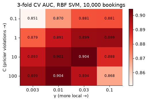
The best combination is C = 10 and $\gamma$ = 0.03, with a cross-validated AUC of 0.904. The worst cell on the grid scores 0.851. Notice the diagonal pattern: when $\gamma$ is large (a very local, wiggly fit), the best C tends to be smaller, and the other way round. That is the interaction in a picture, and the reason not to tune one and then the other.
Look at where the best cell sits in the grid. If it were on the edge, what would you do, and why does it matter?
The best cell is at C = 10, $\gamma$ = 0.03, which is inside the grid, not on its edge. So the search has bracketed the best region: values on either side of it score worse, in both directions. Refining further, between the grid points, would buy a third decimal place, which is noise at this sample size.
The rule is general. A best value on the boundary of the grid tells you only that the answer is at least that extreme. Inside the grid, it tells you that you have found the region. And because cross-validation is itself noisy, the honest reading of a heatmap is “this region is good”, not “this cell is best”.
Now the comparison the chapter has been building to. Same leak-free features, same stratified split and the same 23,878 test bookings as Chapter 12, so the logistic regression’s AUC below is exactly the one reported there.
                                   test AUC  fit seconds
Logistic, all training data           0.889        0.731
Logistic, 10,000 subsample            0.887        0.046
Linear SVM, 10,000 subsample          0.884        0.077
RBF SVM (tuned), 10,000 subsample     0.913        1.583
Three readings.
The tuned RBF SVM ranks bookings best, with a test AUC of 0.913 against 0.889 for Chapter 12’s logistic regression, and it does so having seen only 10,000 of the 95,512 training bookings. The curved boundary is finding structure a linear score cannot: interactions between lead time, the type of customer and the season, say, that logistic regression would need you to type in by hand.
The linear SVM and logistic regression are a dead heat. On the same subsample, their AUCs are 0.884 and 0.887. As the hinge-loss section predicted, when the classes overlap this much, two linear methods with different losses draw nearly the same line. The gain comes from the kernel, not from the hinge.
The kernel is not free. The RBF SVM has 4,110 support vectors, and every prediction compares the new booking with each of them. Scoring the test set took 4.6 seconds, where logistic regression scores it in a blink.
The RBF SVM was trained on 10,000 bookings and logistic regression on all of them. Is that comparison fair? What does the table let you conclude?
It is unfair, but in the SVM’s disfavour, which makes the result stronger. The row that isolates the model is “Logistic, 10,000 subsample”: same data as the SVM, and an AUC of 0.887. Going from 10,000 bookings to all 95,512 raises logistic regression’s AUC by only 0.002: a linear model has few parameters and has learned what it can from 10,000 bookings. The kernel adds 0.026 on the same data. So the gain is the model’s flexibility, not more data.
The obvious next question is what the RBF SVM would do with all the data. The next section explains why that is harder to answer than it sounds.
A kernel SVM has to consider the similarity between pairs of training bookings, and the number of pairs grows with the square of the number of bookings. Double the data and the work roughly quadruples, or worse. Here is the fit time as the training sample grows:
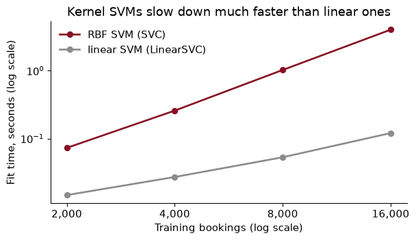
On a log–log plot, the slope of the line is the power at which time grows with $n$. For the RBF SVM it is about 1.9: each doubling of the data multiplies the fit time by about 3.8. Extrapolating that line to the full 95,512 training bookings gives roughly 2 minutes for a single fit, before any tuning, and every one of the grid’s 48 fits would take a similar time. For a card issuer with millions of accounts, kernel SVMs are simply off the table.
Linear SVMs scale in proportion to $n$. scikit-learn’s LinearSVC uses a solver that never forms the pairs, and SGDClassifier(loss="hinge") fits the same hinge-loss model by stochastic gradient descent (Chapter 10), looking at one booking at a time. SGD can even learn from data too big to fit in memory, a batch at a time. On all 95,512 training bookings:
| Model, full training data | Fit seconds | Test AUC |
|---|---|---|
LinearSVC(C=0.1) |
1.2 | 0.887 |
SGDClassifier(loss="hinge") |
0.5 | 0.884 |
| Logistic regression (Chapter 12) | 0.7 | 0.889 |
All three are linear, all three fit in seconds, and all three land within a hair of each other. If you want the kernel’s flexibility at this scale, there are approximations (scikit-learn’s Nystroem builds a few hundred features that mimic the RBF kernel, and a linear SVM is then fitted to those; see Exercise 6). But on large tabular data the more common move is to reach for the trees and boosting of Chapters 14 and 15, which scale well and handle curved boundaries on their own.
Using the fitted slope, how long would one RBF SVM fit take on 32,000 bookings? On 64,000?
The fit on 16,000 bookings took 4.0 seconds. Each doubling multiplies it by 2 raised to the power 1.9, about 3.8, so about 15 seconds at 32,000 and 58 at 64,000. A tuning grid multiplies that again by the number of combinations times the number of folds. This is a rough projection (the exponent changes with the data and the hyperparameters, and large C is slower), but the shape of the answer does not change: kernel methods are for thousands or tens of thousands of cases, not millions.
The hotel’s decision rule from Chapter 12 was: resell a room when the probability of cancellation exceeds $c_{FP}/(c_{FP} + c_{FN}) = 300/400 = 0.75$. That rule needs a probability. The SVM gives a score. On the test set, the tuned RBF SVM’s scores run from -4.4 to 5.9. A score is not a probability, and “resell if the score exceeds 0.75” means nothing.
The AUC did not care, because AUC depends only on the ranking of bookings, and a higher score does mean “more likely to cancel”. But a cost-based threshold, a forecast of empty rooms, or a price all need $\hat p$ to be a number you can multiply by dollars.
The fix is calibration: learn a mapping from scores to probabilities on data the SVM did not train on. The standard method for SVMs is Platt scaling: fit a one-feature logistic regression of the outcome on the SVM’s score. Since the score is already a good ranking, all the little logistic regression has to do is find the S-curve that turns scores into honest frequencies. scikit-learn’s CalibratedClassifierCV does this with cross-validation: it splits the training data into folds, fits the SVM on some and the S-curve on the held-out one, and averages.
cal_svm = CalibratedClassifierCV(make_pipeline(make_prep(), SVC(C=best_C, gamma=best_g)),
                                 method="sigmoid", cv=3).fit(X_sub, y_sub)
p_svm = cal_svm.predict_proba(X_test)[:, 1]
(method="sigmoid" is Platt scaling; "isotonic" fits a more flexible step function and needs more data. You may also see SVC(probability=True), which does the same thing internally. I prefer the explicit wrapper, because it makes clear that the probabilities come from a second model fitted on held-out folds.)
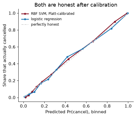
After calibration both models sit close to the diagonal. The calibrated SVM’s Brier score is 0.111, against 0.127 for logistic regression; lower is better. Its AUC is 0.914, slightly different from the uncalibrated 0.913 because the wrapper averages three SVMs fitted on different folds.
Now plug both into Chapter 12’s cost rule, resell when $\hat p > 0.75$, on the test bookings:
| Rule | Share of rooms resold | Average cost per booking (test) |
|---|---|---|
| Never resell | 0% | $37.04 |
| Logistic regression, as in Chapter 12’s cost table | 17% | $23.77 |
| Logistic regression, all training data | 17% | $23.80 |
| RBF SVM, calibrated, 10,000 subsample | 21% | $20.96 |
The SVM’s better ranking turns into money. At the same threshold it resells 21% of rooms rather than 17%, and the average cost per booking is $2.84 lower than logistic regression’s on the same data.
Translate the difference in average cost into dollars per night for a full 200-room hotel. Then say what you would tell the manager about switching models.
The SVM saves $2.84 a booking, so about $567 a night for 200 rooms, or roughly $206,973 a year if every night were like the test set. That is real money for a hotel.
What I would tell the manager: the gain is real but modest, and it comes with costs that do not show up in the table. The SVM cannot be explained in a sentence the way “non-refundable bookings and long lead times cancel more” can. It has to be retrained on a subsample, or replaced by an approximation, as the data grow. Its probabilities come from a second, bolted-on model that must be refitted whenever the SVM is. And Chapter 15’s boosted trees may well do better still, at less cost. So: a strong case for a more flexible model than logistic regression, and a reason to try the tree ensembles before committing to this one.
The whole analysis in one place, from download to a calibrated decision rule, runnable top to bottom. The cleaning and the split are Chapter 12’s.
from pathlib import Path
import numpy as np, pandas as pd
from sklearn.compose import ColumnTransformer
from sklearn.pipeline import make_pipeline
from sklearn.impute import SimpleImputer
from sklearn.preprocessing import StandardScaler, OneHotEncoder
from sklearn.model_selection import train_test_split, GridSearchCV, StratifiedKFold
from sklearn.svm import SVC
from sklearn.calibration import CalibratedClassifierCV
from sklearn.metrics import roc_auc_score
SEED = 368

path = Path("../data/hotels.csv")                    # download once, then reuse
if not path.exists():
    path.parent.mkdir(exist_ok=True)
    pd.read_csv(URL).to_csv(path, index=False)
hotels = pd.read_csv(path)
Drop the leaks and ID-like columns, split exactly as in Chapter 12, and build a preprocessing step that scales the numbers.
LEAKS = ["reservation_status", "reservation_status_date", "assigned_room_type"]
hotels["domestic"] = (hotels["country"] == "PRT").astype(int)
X = hotels.drop(columns=["is_canceled"] + LEAKS + ["agent", "company", "country"])
y = hotels["is_canceled"]
X_train, X_test, y_train, y_test = train_test_split(X, y, test_size=0.2, stratify=y, random_state=SEED)
num = X.select_dtypes("number").columns.tolist()
cat = X.select_dtypes(exclude="number").columns.tolist()
prep = ColumnTransformer([
    ("num", make_pipeline(SimpleImputer(strategy="median"), StandardScaler()), num),
    ("cat", OneHotEncoder(handle_unknown="ignore", sparse_output=False), cat)])
Kernel SVMs need a subsample. Tune C and $\gamma$ together by cross-validated AUC.
X_sub = X_train.sample(10_000, random_state=SEED)
y_sub = y_train.loc[X_sub.index]
grid = {"svc__C": [0.1, 1, 10, 100], "svc__gamma": [0.003, 0.01, 0.03, 0.1]}
search = GridSearchCV(make_pipeline(prep, SVC()), grid, scoring="roc_auc", n_jobs=-1,
                      cv=StratifiedKFold(3, shuffle=True, random_state=SEED)).fit(X_sub, y_sub)
C_star, g_star = search.best_params_["svc__C"], search.best_params_["svc__gamma"]
Calibrate the scores into probabilities, then apply the cost rule once on the test set.
cal = CalibratedClassifierCV(make_pipeline(prep, SVC(C=C_star, gamma=g_star)),
                             method="sigmoid", cv=3).fit(X_sub, y_sub)
p = cal.predict_proba(X_test)[:, 1]
resell, shows_up = p > 0.75, (y_test == 0).values
cost = (300 * (resell & shows_up) + 100 * (~resell & ~shows_up)).mean()
print(f"C = {C_star}, gamma = {g_star} | test AUC {roc_auc_score(y_test, p):.3f} | cost per booking ${cost:.2f}")
C = 10, gamma = 0.03 | test AUC 0.914 | cost per booking $20.96
Forgetting to scale. Without a StandardScaler, the RBF SVM’s AUC on the hotel data drops from 0.900 to 0.697, because lead time and the daily rate swamp every dummy. Scaling is part of the model, so it goes inside the pipeline, learned on the training folds only.
Tuning C and $\gamma$ one at a time, or stopping at the edge of the grid. They interact: the best C depends on $\gamma$. Search them together, on a grid spaced by factors of three or ten. If the best cell is on the edge, extend the grid.
Treating the score as a probability. decision_function returns a signed distance-like score. It ranks bookings, so AUC is fine, but it cannot be compared with 0.75 or summed into a forecast of empty rooms. Calibrate it on held-out data first, and check the reliability curve.
Running a kernel SVM on all the data. Fit time grows roughly with the square of $n$ or faster. On a few thousand cases a kernel SVM is quick; on a hundred thousand, one fit takes minutes and a tuning grid takes an hour or more. Subsample, approximate the kernel, or switch to LinearSVC, SGDClassifier or the tree ensembles of Chapter 15.
Reading ISLP’s $C$ as scikit-learn’s C. In ISLP $C$ is a budget for violations (bigger means a wider street); in scikit-learn it is a price (bigger means a narrower street). Same letter, opposite direction.
Using an SVM when the job is a probability. For pricing insurance, setting a credit limit or forecasting how many rooms will be empty, the probability is the product. Logistic regression gives it directly, and a calibrated SVM gives it second-hand. Use the SVM when the flexible boundary buys enough to pay for the extra step.
Two bookings are on the same side of an SVM’s boundary, with scores 0.4 and 3.1. A colleague proposes to drop the second one from the training data because “it is obviously a cancellation and adds nothing”. If the SVM is refitted without it, does the boundary change? Would the same be true of logistic regression?
A bank fits an SVM to predict loan default and finds that 85% of its training cases are support vectors. What does that tell you about the data? Would you expect a large or small C to have been chosen, and why?
Re-draw the soft-margin figure with the same three values of C, but on the two features lead_time and adr without standardizing them. Describe what happens to the boundary and the street, and explain why.
Extend the tuning grid one step in each direction (C from 0.03 to 300, $\gamma$ from 0.001 to 0.3, still factors of about three). Does the best combination move? Report the best cross-validated AUC and compare it with the original grid’s.
Fit SVC(kernel="poly", degree=2, coef0=1) and SVC(kernel="poly", degree=3, coef0=1) on the 10,000-booking subsample (with C = 1) and compute their test AUC. How do they compare with the linear and RBF SVMs? Which interactions does a degree-2 polynomial kernel let the model use?
Kernel approximation. Build make_pipeline(prep, Nystroem(gamma=best_gamma, n_components=500, random_state=368), LinearSVC(C=0.1)) (import Nystroem from sklearn.kernel_approximation) and fit it on the full training data. Report the fit time and test AUC, and compare them with the RBF SVM trained on 10,000 bookings.
The calibrated SVM resells more rooms than logistic regression at the 0.75 threshold. Using the test set, compute for each model the share of resold rooms whose guest actually shows up (and so is walked). Is the SVM saving money by reselling more rooms at the same accuracy, or by being more accurate about which rooms to resell?
1. For the SVM, no, provided the booking is not a support vector. A score of 3.1 is well past the edge of the street (the edge is at 1), so its hinge loss is zero and it plays no part in setting the boundary. Removing it changes nothing. (The booking with score 0.4 is inside the street, so it is a support vector, and removing it would move the boundary.) For logistic regression, every booking contributes to the log loss, so removing either one moves the coefficients, though removing a confidently correct case moves them very little.
2. That the classes overlap heavily on the features the bank uses: most borrowers sit inside the street or on the wrong side, so most are “hard” cases. Many support vectors usually go with a small C, because cheap violations widen the street and pull more cases into it. It is not a sign of a bug; it is a sign that the features separate defaulters from repayers only weakly, and that the model’s boundary is an average over many ambiguous cases.
3.
X2_raw = np.c_[d2["lead_time"], d2["adr"]]
raw = {C: SVC(kernel="linear", C=C, max_iter=200_000).fit(X2_raw, y2) for C in CS}
fig, ax = plt.subplots(1, 3, figsize=(11, 3.5), sharey=True)
for a, (C, m) in zip(ax, raw.items()):
    plot_svm(a, m, X2_raw, y2, f"unscaled, C = {C}: {len(m.support_)} support vectors")
    a.set_xlabel("lead time (days)")
ax[0].set_ylabel("daily rate (€)"); plt.tight_layout(); plt.show()
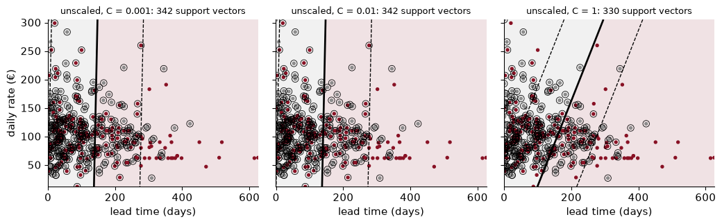
Without scaling, lead time (hundreds of days) and the daily rate (tens to hundreds of euros) are on different scales, and the margin is measured in raw units, so “a wide street” means something different along each axis. The width that the SVM maximises is dominated by whichever feature has the larger spread, and a ridge penalty on the coefficients penalises the two features unequally. The boundaries differ from the scaled ones and depend on the units chosen; quoting the daily rate in cents would change them again. (The max_iter cap is there because the solver struggles on badly scaled data, which is another symptom of the same problem.)
4.
grid2 = {"svc__C": [0.03, 0.1, 0.3, 1, 3, 10, 30, 100, 300], "svc__gamma": [0.001, 0.003, 0.01, 0.03, 0.1, 0.3]}
gs2 = GridSearchCV(make_pipeline(make_prep(), SVC()), grid2, cv=cv3, scoring="roc_auc", n_jobs=-1).fit(X_sub, y_sub)
print(gs2.best_params_, round(gs2.best_score_, 3))
{'svc__C': 10, 'svc__gamma': 0.03} 0.904
The best combination on the wider grid is C = 10, $\gamma$ = 0.03, with a cross-validated AUC of 0.904, against 0.904 on the original grid. The gain is in the third decimal place, well within the noise of 3-fold cross-validation on 10,000 bookings. The lesson is the usual one: the grid needs to bracket the good region, not to be fine.
5.
poly = {deg: make_pipeline(make_prep(), SVC(kernel="poly", degree=deg, coef0=1, C=1)).fit(X_sub, y_sub)
        for deg in [2, 3]}
n_in = make_prep().fit(X_sub).transform(X_sub.head()).shape[1]
poly_auc = {deg: roc_auc_score(y_test, m.decision_function(X_test)) for deg, m in poly.items()}
print({deg: round(a, 3) for deg, a in poly_auc.items()})
{2: 0.906, 3: 0.911}
The degree-2 polynomial kernel has a test AUC of 0.906 and degree 3 has 0.911, against 0.884 for the linear SVM and 0.913 for the tuned RBF. A degree-2 kernel is equivalent to adding every square and every pairwise interaction of the features: lead time × non-refundable, weekend nights × resort hotel, and so on, about 2,080 squares and interactions of the 64 model inputs, that the kernel never has to build. (These polynomial SVMs were not tuned; a fair contest would tune C for each.)
6.
from sklearn.kernel_approximation import Nystroem
nys = make_pipeline(make_prep(), Nystroem(gamma=best_g, n_components=500, random_state=SEED), LinearSVC(C=0.1))
nys, sec_nys = fit_time(nys, X_train, y_train)
auc_nys = roc_auc_score(y_test, nys.decision_function(X_test))
print(f"{sec_nys:.1f} s, test AUC {auc_nys:.3f}")
8.3 s, test AUC 0.916
On all 95,512 training bookings the Nyström approximation fits in 8.3 seconds and reaches a test AUC of 0.916, against 0.913 for the exact RBF SVM on 10,000 bookings and 0.889 for logistic regression. It builds 500 features whose similarities mimic the RBF kernel, using 500 training bookings as landmarks, and then fits a linear SVM to them, so it scales like a linear model. It matches or beats the exact kernel SVM, because it can afford to learn from ten times as many bookings: an approximate kernel on all the data beats an exact one on a tenth of it.
7.
for name, p_ in [("logistic", p_logit_full), ("SVM", p_svm)]:
    r = p_ > 0.75
    print(f"{name}: resells {r.mean():.1%} of rooms; {(y_test.values[r] == 0).mean():.1%} of those guests show up")
logistic: resells 17.1% of rooms; 5.7% of those guests show up
SVM: resells 21.1% of rooms; 6.0% of those guests show up
Of the rooms each model resells, 5.7% (logistic) and 6.0% (SVM) belong to guests who turn up and must be walked. The SVM resells more rooms with almost the same hit rate, so it is mostly finding more of the near-certain cancellations, not gambling more: that is better ranking, which is what its higher AUC promised.
Support vector machines are less common in economics than in computer science, but they had their moment in text classification, and the reviews below explain where they fit among the tools an economist might use.
Antweiler, W. & Frank, M. Z. (2004). “Is All That Talk Just Noise? The Information Content of Internet Stock Message Boards.” Journal of Finance 59(3): 1259–1294. doi.org/10.1111/j.1540-6261.2004.00662.x
The authors collected a very large number of messages posted on internet stock message boards about large US companies and asked whether the chatter predicts anything. They hand-labelled a sample of messages as bullish, bearish or neither, trained text classifiers (Naive Bayes, with a support vector machine as a check) to label the rest, and then related the resulting measures to stock returns, trading volume and volatility. The classifier was not the result, only a way to turn text into a variable.
Think about: the classifier misreads some messages, sarcasm for example. When a mislabelled “bullishness” measure is then used as a regressor, which way does the error push the estimated relationship with returns? Compare that with the hotel, where the classifier’s errors are the final decision.
Gentzkow, M., Kelly, B. & Taddy, M. (2019). “Text as Data.” Journal of Economic Literature 57(3): 535–574. doi.org/10.1257/jel.20181020
A survey of how economists turn documents (newspaper articles, speeches, central bank statements, product reviews) into numbers and use them. It covers how to represent text, how to reduce its huge number of features, and which supervised methods work when there are far more words than documents, a setting where regularised linear classifiers, the family that linear SVMs belong to, tend to do well. Applications range from measuring policy uncertainty to media slant.
Think about: text gives you tens of thousands of features and perhaps a few thousand labelled documents. Why does that setting favour a linear boundary with a penalty over a flexible kernel, and how does it relate to the chapter’s section on linear SVMs for big data?
Athey, S. & Imbens, G. W. (2019). “Machine Learning Methods That Economists Should Know About.” Annual Review of Economics 11(1): 685–725. doi.org/10.1146/annurev-economics-080217-053433
A guided tour, for economists, of the main supervised and unsupervised learning methods, with attention to what they are good at and how they can be adapted to the questions economists care about: causal effects, policy evaluation and inference. It is a good map of where SVMs sit relative to penalised regression, trees, forests and neural networks.
Think about: an SVM gives the hotel a score and a boundary, not a probability or an interpretable coefficient. For the resale decision, what does the hotel lose by not having an honest probability, and when (pricing an overbooking policy, explaining it to a regulator) would that loss matter?
Reading. Géron, Appendix C, for support vector machines, including the dual problem and support vector regression. ISLP (James, Witten, Hastie, Tibshirani & Taylor 2023), ch. 9, for the maximal margin classifier, soft margins (in the budget convention) and the connection to logistic regression. Hsu, Chang & Lin, “A Practical Guide to Support Vector Classification” (National Taiwan University), for the practice of scaling and grid search. Platt (1999), “Probabilistic Outputs for Support Vector Machines”, for the calibration step.