The question: eight numbers describe each country’s health and demography. Is there really a single thing called “development” hiding in them, and if so, how do we measure it?
Economists like to say that a country is “more developed” or “less developed”, as if development were one number. The data never come that way. The CIA World Factbook, in the version distributed by TidyTuesday, gives for each country its birth and death rates, infant and maternal mortality, life expectancy, internet use, net migration and population growth. Keep the 177 countries that report all eight and you have a table with eight columns. Which country is more developed, one with longer lives but slower internet adoption, or the reverse?
The Human Development Index answers by fiat: a committee picks three ingredients and averages them with equal weights. Principal components analysis (PCA) answers from the data: it finds the weighted average of the columns that varies most across countries, and lets you check how much of the table that one average captures. This chapter is about PCA, the workhorse of dimensionality reduction: replacing many correlated variables with a few new ones that keep most of the information.
It is the first method in the book with no outcome variable. Chapters 9 to 15 were supervised: there was a $y$ (rent, cancellation) and we learned to predict it. Here there is only $x$, and the goal is to describe its structure. Chapter 17, on clustering, is the other half of this unsupervised toolkit.
Economists use PCA more than they tend to admit:
Across the 177 countries, the correlation between life expectancy and infant mortality is -0.89, and between net migration and life expectancy it is 0.13. If you had to summarise all eight indicators with one number, which of these two pieces of information would survive, and which would be lost?
Life expectancy and infant mortality are close to mirror images: knowing one, you nearly know the other, so a single “development” score can carry both with little loss. Net migration is almost unrelated to life expectancy, so it is telling you something else (where people are moving, which depends on wars, oil money and labour markets, not only on health). One number cannot carry two unrelated pieces of information; the second needs a second dimension. That is the whole logic of PCA in one sentence: correlated columns can be compressed, uncorrelated ones cannot.
Why bother reducing dimensions at all? Partly for interpretation: eight columns are hard to think about, one or two are easy. But there is a deeper reason, and it bites every method in this book that relies on distances.
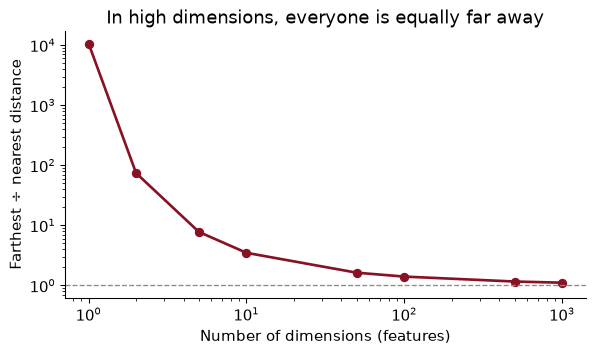
Recall nearest neighbours from Chapter 9: to predict the rent of a flat, find the most similar flats and average their rents. “Most similar” means “closest”, and closeness behaves strangely when there are many dimensions. Scatter 500 points at random in a cube, and for each point compare the distance to its farthest neighbour with the distance to its nearest one:
from scipy.spatial.distance import pdist, squareform
rng = np.random.default_rng(368)
ratio = {}
for d in [2, 10, 100, 1000]:
    D = squareform(pdist(rng.uniform(size=(500, d))))       # all pairwise distances
    np.fill_diagonal(D, np.nan)
    ratio[d] = np.nanmean(np.nanmax(D, 1) / np.nanmin(D, 1))   # farthest / nearest, averaged
print({d: round(r, 2) for d, r in ratio.items()})
{2: np.float64(91.21), 10: np.float64(3.45), 100: np.float64(1.4), 1000: np.float64(1.11)}
In two dimensions the farthest point is, on average, 91 times as far away as the nearest. In 100 dimensions the ratio is 1.40; in 1,000 it is 1.11. Distances concentrate: every point is roughly the same distance from every other, so “nearest” stops meaning “similar”. This is the curse of dimensionality.
There is a second way to see it. To capture 10% of the points in a unit cube by taking a smaller cube around one of them, the small cube needs an edge of $0.1^{1/d}$. In one dimension that is 0.1, a genuinely local neighbourhood. In ten dimensions it is 0.79: to find 10% of the data you must reach across most of the range of every variable. Neighbourhoods stop being local.
For an economist this is not abstract. Matching estimators find, for each treated person, the most similar untreated person. With age and education, that is easy. With fifty covariates, nobody is similar to anybody, and the matches are poor. The cure is the same in both settings: find the few directions in which the data really vary, and work there. Real data, unlike random points in a cube, nearly always have such directions, because real variables are correlated.
You want a neighbourhood containing 1% of the data, using a cube around a point in a unit cube with $d$ dimensions. How long must its edge be when $d$ = 2, 10, and 50?
The edge is $0.01^{1/d}$: 0.10 for $d$ = 2, 0.63 for $d$ = 10, and 0.91 for $d$ = 50. With fifty features, a “neighbourhood” holding 1% of the data spans more than nine-tenths of the range of every feature. It is not a neighbourhood at all, and a nearest-neighbour prediction made from it is really an average over very different cases.
Start with two columns, life expectancy and infant mortality, each standardized (minus its mean, divided by its standard deviation) so that both are measured in standard deviations. The left panel below plots them. The points lie along a line sloping down: countries where babies die are countries where adults die young.
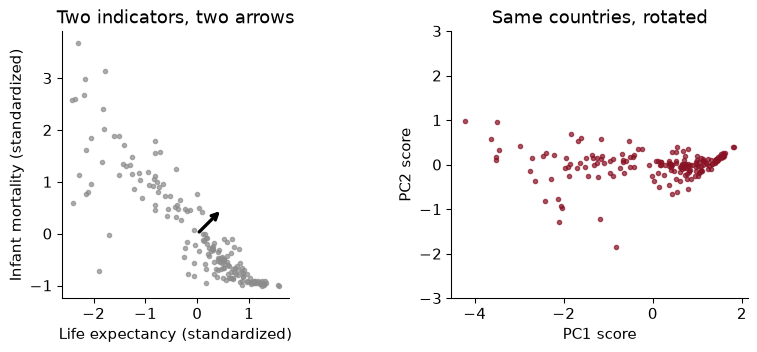
PCA asks: along which direction are the points most spread out? That is the garnet arrow, the first principal component (PC1). Then: at right angles to it, which direction has the most remaining spread? That is the black arrow, PC2. With two variables there is nothing left to choose; with eight, PCA keeps going, each new direction at right angles to all the previous ones. Then it rotates the data so that the new directions are the axes, which is the right panel. Nothing is lost by rotating. Something is lost only when you decide to keep fewer components than you started with.
Here, PC1 accounts for 94% of the total variance of the two standardized columns. Throw PC2 away and you keep almost all the information in one number.
Now the one equation. A principal component score for country $i$ is a weighted sum of its standardized variables:
\[z_{i1} = \phi_{1}\, x_{i1} + \phi_{2}\, x_{i2} + \dots + \phi_{p}\, x_{ip}\]The weights $\phi$ are the loadings. PC1’s loadings are the ones that make the scores $z_{i1}$ as spread out across countries as possible, subject to the squared weights adding to one (otherwise you could inflate the spread just by doubling every weight). PC2’s loadings do the same, subject also to PC2’s scores being uncorrelated with PC1’s. The loadings tell you what a component means; the scores tell you where each country sits on it.
Going further. If $\Sigma$ is the correlation matrix of the standardized data, PC1’s loadings solve $\max_{\phi} \phi^\top \Sigma \phi$ subject to $\phi^\top\phi = 1$. The solution is the eigenvector of $\Sigma$ with the largest eigenvalue, and that eigenvalue is the variance of the PC1 scores. Software computes all of them at once from the singular value decomposition of the data matrix. You will never need to do it by hand, but it is why PCA always gives the same answer: there is no random start and no tuning.
For the two-variable PCA, PC1’s loadings are 0.707 on life expectancy and -0.707 on infant mortality. Brazil’s standardized values are 0.299 and -0.316. What is its PC1 score, and what does the sign mean?
Multiply and add: 0.707 × 0.299 + (-0.707) × -0.316 = 0.435, which matches PCA().transform (0.435). The loadings have opposite signs, so PC1 is “long lives and few infant deaths” at one end and the reverse at the other. Which end is positive is arbitrary: flip both loadings and every score changes sign, and the component explains exactly the same variance. Read signs from the loadings, never assume them.
PCA chases variance, and variance depends on units. In the Factbook, maternal mortality is measured in deaths per 100,000 births, with a standard deviation across countries of 222. Internet use is a share, with a standard deviation of 0.27. Run PCA on the raw numbers and see what happens:
PCA().fit(df[FEAT]).components_[0].round(3) # PC1 loadings, unstandardized
array([ 0.035, 0.005, 0.095, -0.001, -0.032, 0.994, -0.004, 0.003])
PC1 puts a loading of 0.994 on maternal mortality and almost nothing on anything else, and it “explains” 99.3% of the variance. That is not a discovery about development. It is a discovery that 222 is bigger than 0.27. Measure maternal mortality per 1,000 births instead and the answer would change completely.
So standardize before PCA unless every variable is in the same, meaningful unit. Standardizing gives each variable a variance of one, so each gets an equal say before PCA decides which combinations matter. The exception, which we meet with interest rates, is when all the columns share a unit and the differences in their variances are real information.
Which of these should be standardized before PCA? (a) Monthly returns on 30 stocks, all in percent. (b) A household survey with income in dollars, years of schooling, and number of children. (c) Yields on seven Treasury bonds, all in percent.
(b), certainly: dollars and years are not comparable, and unstandardized PCA would return “income”. (a) and (c) are judgement calls, and the usual practice is not to standardize. All the columns are in the same unit, and if one stock is more volatile than another, that volatility is exactly what a portfolio manager cares about. Standardizing would give a sleepy utility stock the same weight as a volatile tech stock. With interest rates, short rates genuinely move more than long rates, and we want PCA to see that.
Eight standardized indicators carry eight units of variance in total, one each. PCA re-divides that total among the components, largest first. The share each captures is its explained variance ratio, and a bar chart of them is a scree plot (scree is the rubble at the foot of a cliff, which is what the small components look like).
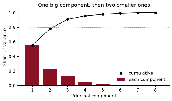
PC1 alone captures 56% of the variance in the eight indicators. PC2 adds 22% and PC3 13%; together the first three hold 91%. After that the bars are rubble.
How many to keep has no single right answer. Common rules are to keep enough for 80% or 90% of the variance (here 3 components reach 80%), or to cut at the “elbow” where the bars flatten, or to keep components with more variance than an average original variable (an eigenvalue above one, in the standardized case). In practice the purpose decides. For an index, one component; for a picture, two; as inputs to a regression, as many as cross-validation likes (later in the chapter).
A classmate says: “PC1 explains 56%, so development is about half of what varies between countries, and the other half is noise.” Is that right?
The first half is a fair reading; the second is not. The remaining 44% is not noise. PC2 and PC3 together carry 35% of the variance, and as the next section shows, they have clear meanings of their own. “Explained variance” is a statement about the eight columns we chose to include, too: add five more health indicators and PC1’s share would rise, add five unrelated ones and it would fall. The share describes the table, not the world.
The loadings say what each component is made of. I orient each one so that life expectancy loads positively, which only flips signs and changes nothing else:
                          PC1   PC2   PC3
birth_rate              -0.44  0.04  0.20
death_rate              -0.15 -0.36 -0.79
infant_mortality_rate   -0.45 -0.06  0.00
internet_pc              0.37 -0.03 -0.36
life_exp_at_birth        0.45  0.14  0.10
maternal_mortality_rate -0.43 -0.07 -0.12
net_migration_rate       0.01  0.66 -0.43
population_growth_rate  -0.25  0.63 -0.05
PC1 is development. Life expectancy and internet use load positively; birth rates, infant mortality and maternal mortality load negatively, all with similar weights. It is the familiar demographic transition, from high fertility and high mortality to low fertility and long lives, read straight out of the data.
PC2 is migration and growth. It is dominated by net migration and population growth, loading together. Countries high on PC2 are gaining people, either by births or by arrivals; those low on it are losing them.
PC3 is mostly the death rate, once the other components have taken what they can. That sounds odd until you remember that the crude death rate depends on age structure: a rich, old country like Japan and a poor, young one can have similar death rates for opposite reasons. PC1 had to handle “poor countries die young” and could not also handle “old countries die more”; PC3 picks up the second.
A biplot shows countries (points) and loadings (arrows) together on the first two components:
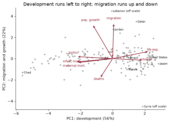
Rich, ageing countries sit on the right with low PC2; the poorest and youngest on the left. The countries far up the PC2 axis are Lebanon, by a wide margin, and Jordan, which took in refugees from Syria’s civil war, along with Gulf states such as Qatar whose populations are swollen by migrant workers. Syria itself sits far below everyone else. That is a real feature of the world which a one-dimensional development index would miss entirely.
Without looking at the data, a colleague guesses that PC2 is “being rich but not healthy”. What would you check to test the guess, and what does the table say?
Check the loadings: a “rich but unhealthy” component would load positively on internet use and positively on mortality. PC2 does neither in any strong way. Its two large loadings are net migration (0.66) and population growth (0.63), with everything else small. Then check the countries at the extremes of the scores: the top of PC2 is Lebanon and Jordan (refugee inflows) and the Gulf states (migrant workers), and the bottom is Syria, so “migration” is the better name. Naming a component is a hypothesis about its loadings and its extreme cases, and you should check both.
PC1’s scores are a development index built by the data. Here are the ten lowest and ten highest countries:
                  lowest  score       highest  score
                    Chad   -5.61        Japan   2.85
                 Somalia   -5.61 Korea, South   2.67
Central African Republic   -5.10      Iceland   2.65
                    Mali   -4.99  Netherlands   2.61
             Afghanistan   -4.91      Germany   2.55
           Guinea-Bissau   -4.84    Singapore   2.53
                   Niger   -4.83       Sweden   2.50
            Sierra Leone   -4.41  Switzerland   2.50
                 Burundi   -4.23       Norway   2.47
                  Zambia   -4.04      Finland   2.47
The bottom of the list is the Sahel and Central Africa; the top is Japan, Western Europe and the rich East Asian economies. No one told PCA about income, region or history, and it produced a ranking that any development economist would recognise. The index correlates 0.94 with life expectancy and 0.79 with internet use.
Two cautions. First, it is a descriptive index of these eight indicators, from an older edition of the Factbook; it is not GDP and not welfare, and it inherits whatever the eight indicators leave out (income, inequality, freedom). Second, the weights are chosen to maximise variance, not to reflect anyone’s values. If you think infant mortality matters more than internet use, PCA will not respect that. The HDI’s equal weights are arbitrary too, but they are arbitrary in public, by a choice someone can defend or criticise. PCA’s weights are data-driven, which is not the same as neutral.
The index and life expectancy are correlated at 0.94. If they agree that closely, why build an index at all?
Because a correlation of 0.94 still leaves room for large disagreements about individual countries, and for some purposes those are what matter. The biggest is Syria: 121st by life expectancy, 36th by the index. At the other end, Lebanon is 43rd by life expectancy but 112th by the index. Both moves come from the migration columns, which PC1 weights lightly but not at zero: a population shrinking through emigration nudges the index up, and one swelling with refugees nudges it down. That is a reminder to read an index’s loadings before trusting its rankings. An index averages over several noisy indicators, so a country’s position does not hinge on one statistic that may be badly measured. That is the same reason we prefer a test score built from many questions to a score on one question.
Now a setting where the columns share a unit. FRED publishes daily yields on US Treasury securities at many maturities, free and without an API key. Take seven, from three months to ten years, and average them by month: 542 months from September 1981 to October 2026.
FRED = "https://fred.stlouisfed.org/graph/fredgraph.csv?id=DGS3MO,DGS1,DGS2,DGS3,DGS5,DGS7,DGS10"
ypath = Path("../data/treasury_yields.csv")                 # download once, then reuse
if not ypath.exists():
    pd.read_csv(FRED, na_values=".").to_csv(ypath, index=False)
yields = (pd.read_csv(ypath, parse_dates=["observation_date"], index_col="observation_date")
          .resample("ME").mean().dropna())
yields.columns = ["3m", "1y", "2y", "3y", "5y", "7y", "10y"]
dy = yields.diff().dropna()               # monthly changes, percentage points
pca_y = PCA().fit(dy)                     # same units: no standardizing
I run PCA on monthly changes, because that is what moves bond prices and what a trader hedges; and I do not standardize, because all seven are in percentage points and the extra volatility of short rates is real. The result is one of the cleanest in empirical economics. PC1 explains 87.3% of the variance of yield changes, PC2 10.4% and PC3 1.7%: three components, 99.3% of everything that happens to the yield curve.
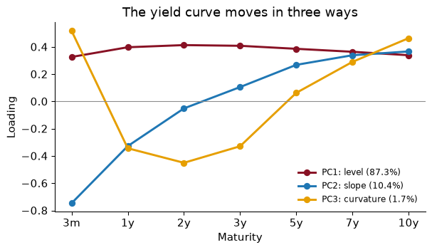
The loadings have a shape you can name at a glance:
Litterman and Scheinkman (1991) found these three factors in the early 1990s, and bond desks still hedge them: a portfolio protected against level, slope and curvature is protected against nearly everything rates do.
The slope factor has an economic payoff. Fit the same PCA to the levels of yields and plot PC2’s score over time next to the term spread, the 10-year yield minus the 3-month:
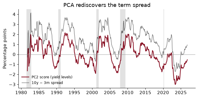
The two lines are almost the same, with a correlation of 0.996. PCA was told nothing about spreads, recessions, or which maturity is which; it found the slope because the slope is how the curve actually moves. And the term spread is one of the best-known recession predictors in macroeconomics: it has turned negative (an “inverted” curve) before each of the recessions shaded in the chart.
A one-standard-deviation move in the level component, in a typical month, shifts each yield by its loading times the component’s standard deviation (0.73 percentage points). How much do the 3-month and 10-year yields move?
The 3-month yield moves by 0.33 × 0.73 = 0.24 points and the 10-year by 0.34 × 0.73 = 0.25 points: roughly 24 and 25 basis points. “Level” does not mean every yield moves by exactly the same amount; the loadings are similar, not equal. A bond trader who wants to be immune to level shocks weights her positions so that their sensitivities, multiplied by these loadings, sum to zero.
Principal components can also be inputs to a regression. Principal components regression (PCR) replaces the $p$ original features with their first $M$ component scores and runs OLS on those. With $M = p$ it is exactly OLS; with smaller $M$ it throws away the low-variance directions, which reduces variance at the cost of some bias, the same trade as ridge regression in Chapter 11. Stock and Watson’s diffusion-index forecasts are PCR on a large macro panel.
To try it here, predict life expectancy from the other seven Factbook indicators, choosing $M$ by five-fold cross-validation (Chapter 9):
components M
1    3.78
2    3.15
3    2.91
4    2.86
5    2.81
6    2.81
7    2.83
One component already predicts life expectancy to within 3.8 years (its standard deviation across countries is 8.8), because PC1 of the other seven indicators is mostly the development axis, and life expectancy lives on it. The best cross-validated choice is $M$ = 5, with an RMSE of 2.81, against 2.83 for OLS on all seven: a small gain, from dropping noisy directions.
The caveat is the important part. PCA chooses components without looking at $y$. The directions in which the features vary most need not be the directions that predict the outcome. Here they happen to be, because life expectancy is part of the same demographic story; in other problems the top components predict nothing and the useful signal sits in a small component that PCR throws away. Ridge and LASSO (Chapter 11) look at $y$ and are usually the safer default.
With $M = 7$, PCR’s cross-validated RMSE is 2.828 and OLS’s is 2.828. Coincidence?
No. With all seven components, PCR has only rotated the features, and OLS on a rotation of the features gives exactly the same fitted values as OLS on the features themselves: the same column space, the same projection. Dimensionality reduction starts only when $M < p$. This is a useful check that your pipeline is wired correctly.
The first two components make a decent map of high-dimensional data: here they hold 78% of the variance. But PCA is linear; it can only rotate and flatten. t-SNE (van der Maaten and Hinton 2008) is a popular non-linear alternative that tries to place points so that each one’s nearest neighbours in the original space stay near it on the page. It is very good at showing local groups:
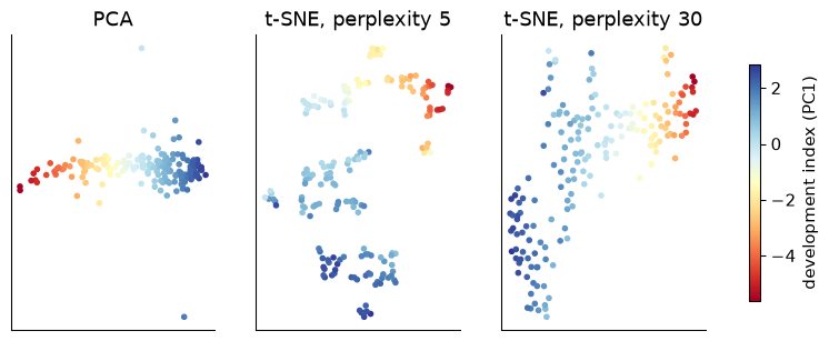
The PCA map is a straight development gradient. The t-SNE maps break the same countries into islands, and the islands depend on the perplexity, a tuning parameter that sets roughly how many neighbours each point cares about. Neither t-SNE map is wrong. Both are answers to a vaguer question than PCA’s.
The rules for reading t-SNE, which matter because the pictures are so persuasive:
transform for new data. You cannot say what an axis means, and you should never feed t-SNE coordinates into a regression.My rule of thumb: PCA to measure and compress, t-SNE to look. In this book, t-SNE’s natural home is Chapter 20, where documents and words live in hundreds of dimensions and a picture of who is near whom is genuinely useful. UMAP, a faster cousin, has the same caveats.
In the perplexity-5 map, a student spots a small island well separated from the rest and writes: “these countries form a distinct development type, very different from all the others.” What can and cannot be concluded?
What can be concluded: those countries are each other’s nearest neighbours in the eight-dimensional data, so they are similar to one another. What cannot: that they are very different from the rest. t-SNE does not preserve distances between groups, and a smaller perplexity tends to cut the data into more, tighter islands, so the gap on the page says more about the setting than about the countries. To check, go back to the data: compare the island’s average indicators with everyone else’s, or look at where those countries fall on PCA’s map, where distances do mean something. Clustering, in Chapter 17, gives a more disciplined way to ask whether groups exist.
The whole analysis, runnable top to bottom: the Factbook index, then the yield curve.
from pathlib import Path
import numpy as np, pandas as pd
from sklearn.decomposition import PCA
from sklearn.preprocessing import StandardScaler

path = Path("../data/cia_factbook.csv")                     # download once, then reuse
if not path.exists():
    path.parent.mkdir(exist_ok=True)
    pd.read_csv(CIA_URL).to_csv(path, index=False)
cia = pd.read_csv(path)
cia["internet_pc"] = cia["internet_users"] / cia["population"]   # a count is not comparable
FEAT = ["birth_rate", "death_rate", "infant_mortality_rate", "internet_pc", "life_exp_at_birth",
        "maternal_mortality_rate", "net_migration_rate", "population_growth_rate"]
df = cia.dropna(subset=FEAT).set_index("country")
Standardize, fit, and orient PC1 so that higher means longer lives.
Z = StandardScaler().fit_transform(df[FEAT])
pca = PCA().fit(Z)
print("explained variance:", pca.explained_variance_ratio_.round(3))
sign = np.sign(pca.components_[0][FEAT.index("life_exp_at_birth")])
loadings = pd.DataFrame(sign * pca.components_[:2].T, index=FEAT, columns=["PC1", "PC2"])
dev_index = pd.Series(sign * pca.transform(Z)[:, 0], index=df.index).sort_values()
print(loadings.round(2)); print(dev_index.tail(5).round(2))
explained variance: [0.556 0.223 0.129 0.048 0.023 0.013 0.008 0.   ]
                          PC1   PC2
birth_rate              -0.44 -0.04
death_rate              -0.15  0.36
infant_mortality_rate   -0.45  0.06
internet_pc              0.37  0.03
life_exp_at_birth        0.45 -0.14
maternal_mortality_rate -0.43  0.07
net_migration_rate       0.01 -0.66
population_growth_rate  -0.25 -0.63
country
Germany         2.55
Netherlands     2.61
Iceland         2.65
Korea, South    2.67
Japan           2.85
dtype: float64
The yield curve: PCA on monthly changes, no standardizing.
yields = (pd.read_csv(ypath, parse_dates=["observation_date"], index_col="observation_date")
          .resample("ME").mean().dropna())
yields.columns = ["3m", "1y", "2y", "3y", "5y", "7y", "10y"]
pca_y = PCA(3).fit(yields.diff().dropna())
print("explained variance:", pca_y.explained_variance_ratio_.round(3))
print(pd.DataFrame(pca_y.components_.T, index=yields.columns,
                   columns=["level", "slope", "curvature"]).round(2))
explained variance: [0.873 0.104 0.017]
     level  slope  curvature
3m    0.33   0.75       0.52
1y    0.40   0.33      -0.34
2y    0.41   0.05      -0.45
3y    0.41  -0.11      -0.33
5y    0.39  -0.27       0.06
7y    0.36  -0.34       0.29
10y   0.34  -0.37       0.46
Principal components regression, with the number of components chosen by cross-validation.
from sklearn.pipeline import make_pipeline
from sklearn.linear_model import LinearRegression
from sklearn.model_selection import GridSearchCV, KFold
X, y = df[[f for f in FEAT if f != "life_exp_at_birth"]], df["life_exp_at_birth"]
pcr = make_pipeline(StandardScaler(), PCA(), LinearRegression())
grid = GridSearchCV(pcr, {"pca__n_components": range(1, 8)}, cv=KFold(5, shuffle=True, random_state=368),
                    scoring="neg_root_mean_squared_error").fit(X, y)
print(grid.best_params_, round(-grid.best_score_, 2))
{'pca__n_components': 5} 2.81
Forgetting to standardize. Unstandardized PCA on the Factbook put a loading of 0.99 on maternal mortality, because it is measured in the biggest units. Standardize whenever the columns are in different units, and think before standardizing when they are not.
Reading the sign of a component. Software may return PC1 with “development” pointing either way, and a different version of the library may flip it. Orient components deliberately (here, so that life expectancy loads positively) and say so.
Treating explained variance as importance. A component that explains 2% of the variance can be the one that matters for your question; in the yield curve, curvature is 1.7% of the variance and still something traders hedge. And PCR’s top components are not guaranteed to predict anything, because PCA never looked at $y$.
Fitting PCA on the test set. PCA is a learned transformation like a scaler. In a prediction problem, fit it inside the pipeline on training data only, exactly as in Chapter 9, or information from the test set leaks into the features.
Over-reading a t-SNE map. Cluster sizes and distances between clusters are not meaningful, and the picture changes with the perplexity. Use t-SNE to look and PCA (or the original variables) to measure.
Forgetting what went in. PCA describes the columns you chose. A “development index” built from eight demographic and health indicators says nothing about income, inequality or institutions, and its weights are chosen to maximise variance, not to reflect anyone’s values.
A country’s PC1 score is 0 in the standardized Factbook PCA. What does that mean? Which of these is right: (a) it has average values on all eight indicators; (b) its weighted combination of standardized indicators equals the average country’s; (c) it is exactly in the middle of the development ranking?
Compute the correlation matrix of the eight Factbook indicators and find the pair with the strongest correlation. How does that fit with PC1’s loadings?
Drop net_migration_rate and population_growth_rate, refit the standardized PCA on the remaining six indicators, and report the share of variance PC1 explains. Explain why it rose.
Rebuild the development index using log of maternal and infant mortality instead of their raw values. Which countries move most in the ranking?
Run the yield-curve PCA on monthly changes for the period from January 2008 onwards only. Do level, slope and curvature survive, and how do their shares change?
Using the curse-of-dimensionality simulation, compute the standard deviation of all pairwise distances divided by their mean, for 2, 10, 100 and 1,000 dimensions. What happens, and why does it matter for nearest neighbours?
Fit t-SNE on the standardized Factbook data with perplexity 30, init="random", and two different seeds. Do the two maps look the same? What does that tell you?
1. (b). A PC1 score is a weighted sum of standardized values, so zero means the weighted sum equals that of a country with every indicator at its mean. That does not require (a): a country can be above average on some indicators and below on others in a way that cancels. Nor (c): the scores are not symmetric, so zero need not be the median.
countries with a PC1 score below zero: 40%
In fact 40% of countries have a negative development score, so zero is not the middle of the ranking.
2.
corr = df[FEAT].corr()
pairs = corr.where(np.triu(np.ones(corr.shape, dtype=bool), k=1)).stack()
print(pairs.abs().sort_values(ascending=False).head(3).round(3))
infant_mortality_rate  life_exp_at_birth          0.887
birth_rate             infant_mortality_rate      0.865
infant_mortality_rate  maternal_mortality_rate    0.857
dtype: float64
The strongest pair is infant_mortality_rate and life_exp_at_birth, with a correlation of -0.89. Both have large PC1 loadings (-0.45 and 0.45). Strongly correlated variables are exactly what PC1 bundles together: one direction can describe both.
3.
six = [f for f in FEAT if f not in ("net_migration_rate", "population_growth_rate")]
evr6 = PCA().fit(StandardScaler().fit_transform(df[six])).explained_variance_ratio_
print(evr6.round(3))
[0.704 0.178 0.062 0.029 0.017 0.011]
PC1 now explains 70% of the variance of the six indicators, up from 56% with eight. The two dropped variables were the ones PC1 did not capture (they formed PC2), so removing them leaves a table that is more nearly one-dimensional. This is the warning from the scree section in action: explained variance describes the columns you chose.
4.
logged = df[FEAT].assign(maternal_mortality_rate=np.log(df["maternal_mortality_rate"]),
                         infant_mortality_rate=np.log(df["infant_mortality_rate"]))
pl = PCA().fit(StandardScaler().fit_transform(logged))
s_log = pl.transform(StandardScaler().fit_transform(logged))[:, 0]
s_log *= np.sign(pl.components_[0][FEAT.index("life_exp_at_birth")])
shift = (pd.Series(s_log, index=df.index).rank() - dev.reindex(df.index).rank()).sort_values()
print(shift.head(3), shift.tail(3))
country
Syria                              -21.0
Saint Vincent and the Grenadines   -14.0
Saint Lucia                        -12.0
dtype: float64 country
Russia     17.0
Ukraine    20.0
Belarus    22.0
dtype: float64
The two indices correlate at 0.975, so the broad ranking is unchanged. The biggest risers under the logged version are Belarus, Ukraine, Russia, and the biggest fallers Syria, Saint Vincent and the Grenadines, Saint Lucia. Logging compresses the differences among very high mortality rates and stretches those among low ones, so the countries that move most are those whose mortality rates are low relative to their other indicators (they gain) or high relative to them (they lose). Any index is a set of choices; it is worth knowing which ones move the answer.
5.
recent = yields.loc["2008-01-01":].diff().dropna()
pca_r = PCA(3).fit(recent)
print(pca_r.explained_variance_ratio_.round(3))
print(pd.DataFrame(pca_r.components_.T, index=yields.columns).round(2))
[0.813 0.142 0.033]
        0     1     2
3m   0.23  0.67  0.57
1y   0.32  0.45 -0.10
2y   0.37  0.20 -0.48
3y   0.41  0.04 -0.42
5y   0.44 -0.22 -0.06
7y   0.43 -0.33  0.21
10y  0.41 -0.38  0.46
Since 2008 the first three components explain 81.3%, 14.2% and 3.3% of the variance of yield changes, against 87.3%, 10.4% and 1.7% over the full sample. The level share is smaller and the slope share larger: for much of the period short rates were pinned near zero, so a lot of the action was in long rates alone, which looks like a change in slope. The shapes of the loadings are the familiar three, which is why practitioners trust them.
6.
rng = np.random.default_rng(368)
cv_dist = {d: (lambda D: D.std() / D.mean())(pdist(rng.uniform(size=(500, d)))) for d in [2, 10, 100, 1000]}
print({d: round(float(v), 3) for d, v in cv_dist.items()})
{2: 0.477, 10: 0.192, 100: 0.059, 1000: 0.019}
The relative spread of distances falls from 0.48 in two dimensions to 0.019 in 1,000. When all distances are nearly equal, the “nearest” neighbour is barely nearer than a random point, so a nearest-neighbour prediction is close to an average over everyone. That is the curse: methods built on distance lose their meaning as the number of features grows, unless the data really live in a few dimensions.
7.
from scipy.stats import spearmanr
from scipy.spatial.distance import pdist
e1 = TSNE(2, perplexity=30, init="random", random_state=1).fit_transform(Z)
e2 = TSNE(2, perplexity=30, init="random", random_state=2).fit_transform(Z)
rho_d = spearmanr(pdist(e1), pdist(e2)).statistic
The two maps differ in layout (islands can be rotated, reflected, or placed differently), and the rank correlation between their pairwise distances is 0.98. Who is close to whom is broadly stable; the overall arrangement is partly an accident of the run. That is the right way to use t-SNE: trust the local neighbourhoods that persist across seeds and settings, and nothing else.
Principal components are the standard way economists summarise many correlated series. These papers apply them to macroeconomic forecasting and to the yield curve of this chapter.
Litterman, R. B. & Scheinkman, J. (1991). “Common Factors Affecting Bond Returns.” Journal of Fixed Income 1(1): 54–61. doi.org/10.3905/jfi.1991.692347
The paper behind the level, slope and curvature section. Litterman and Scheinkman apply factor analysis to returns on US Treasury bonds of different maturities and find that three factors account for nearly all of their movement: a shift of the whole curve, a tilt between short and long rates, and a bend in the middle. Bond traders and central banks have used that description ever since to measure and hedge interest-rate risk.
Think about: the factors are statistical, but economists give them economic names. What might move the “level” factor (expected inflation, say) and what might move the “slope” (the stance of monetary policy)? Why is naming a component an economic argument rather than something the PCA tells you?
Stock, J. H. & Watson, M. W. (2002). “Forecasting Using Principal Components From a Large Number of Predictors.” Journal of the American Statistical Association 97(460): 1167–1179. doi.org/10.1198/016214502388618960
Macroeconomists have hundreds of monthly series and only a few hundred months. Stock and Watson summarise a large panel of US series with a handful of principal components and use those components to forecast output and inflation. Forecasts built on the components beat standard benchmarks, because a few common factors carry most of what the many series know about the economy. This is principal components regression, the chapter’s short section, at national scale.
Think about: the components are chosen to explain the predictors, not the variable you want to forecast. When could the first few components of a big macro data set be useless for forecasting inflation, and how would you find out?
McCracken, M. W. & Ng, S. (2016). “FRED-MD: A Monthly Database for Macroeconomic Research.” Journal of Business & Economic Statistics 34(4): 574–589. doi.org/10.1080/07350015.2015.1086655
The authors built a freely available, regularly updated monthly database of more than a hundred US macroeconomic series, hosted on FRED, along with the transformations needed to make each one roughly stationary. They extract principal components from it and show that the first few line up with recognisable aspects of the economy such as real activity, prices and interest rates.
Think about: the chapter calls PC1 of the Factbook data a development index. If you found that PC1 of FRED-MD tracks the business cycle, what checks would you want before using it as an “index of economic activity”, and what would you do about series that are missing in early years?
Reading. Géron, ch. 7, for PCA, its randomized and incremental variants, and other dimensionality-reduction methods. ISLP (James, Witten, Hastie, Tibshirani & Taylor 2023), §12.2, for PCA, and §6.3 for principal components regression. Litterman & Scheinkman (1991), “Common Factors Affecting Bond Returns”, for level, slope and curvature; Stock & Watson (2002), “Forecasting Using Principal Components from a Large Number of Predictors”, for factor models in macroeconomics.