The question: central banks, landlords and newspapers all publish words, not numbers. How do you turn those words into a variable you can put in a regression, and how do you know the variable measures what you claim it measures?
Most of what happens in an economy is written down before it is counted. The Federal Open Market Committee (FOMC) releases a statement after every meeting, minutes three weeks later, and transcripts five years later. Firms file 10-Ks and hold earnings calls. Every rental flat in San Francisco was, for most of the 2000s, advertised in a one-line Craigslist title. Newspapers report on all of it. None of this arrives as a column in a spreadsheet.
Economists used to read such text and code it by hand. That still happens, and it is still the gold standard, but it does not scale: you can read 500 FOMC sentences in an afternoon, not 5 million newspaper articles. Text as data is the set of methods for doing the reading by machine.
Gentzkow, Kelly and Taddy (2019) describe every text project with the same three steps, and I find their notation worth learning because it makes you say what you are doing:
There are four broad ways to do step 2. A dictionary method counts words from a list someone wrote down. A supervised method learns which words matter from documents that humans have already labelled. A topic model finds groups of words that travel together, with no labels at all. And embeddings and language models replace word counts with dense learned vectors. This chapter does the first two. Chapter 20 does topics and embeddings, and Chapter 21 does transformers and large language models.
The thing to hold on to throughout is that $\hat V$ is a measurement. It has error, and its error may be correlated with the things you later put on the right-hand side. Most of the hard thinking in a text project goes into convincing yourself, and a referee, that $\hat V$ measures $V$.
For each project, name $\mathcal{D}$, $\hat V$, and whether the measurement step is a dictionary or supervised. (a) Baker, Bloom and Davis (2016) count newspaper articles that mention the economy, policy and uncertainty. (b) A researcher has 2,000 FOMC sentences that economists have labelled hawkish or dovish, and wants to score the other 50,000. (c) A housing office wants to know how much the words in a rental ad add to the predicted rent.
(a) $\mathcal{D}$ is newspaper articles; $\hat V$ is the share of articles each month about economic policy uncertainty; the method is a dictionary, three short word lists chosen by the authors. (b) $\mathcal{D}$ is FOMC sentences; $\hat V$ is each sentence’s stance; supervised, because the labelled sentences teach the model which words signal hawkishness. (c) $\mathcal{D}$ is ad titles; $\hat V$ is the predicted (log) rent; supervised, with the observed rent as the label. Notice that in (c) the label is a number we already have for every ad. We are not trying to measure rent, which we observe; we are asking what the text knows about rent beyond the structured columns.
Before any counting, text usually needs cleaning, and the tool for that is the regular expression, or regex: a small language for describing patterns in strings. You have already met pandas’ .str methods; regex is what goes inside them.
Five pieces cover most of what an economist needs. \d is a digit, \w a letter, digit or underscore, \s a space. + means “one or more”, * “zero or more”, ? “optional”. Square brackets give a set, so [Ss]ales matches both capitalisations. \b is a word boundary, so \bfed\b matches “fed” but not “federal”. Parentheses capture a piece you want to keep. Always write patterns as raw strings, r"...", so Python does not eat the backslashes, and test them at regex101.com before trusting them.
Here is a sentence from a 2023 FOMC statement, and a pattern that pulls out the target range for the federal funds rate:
stmt = ("The Committee decided to maintain the target range for the federal funds "
        "rate at 5-1/4 to 5-1/2 percent.")
m = re.search(r"(\d+)-(\d)/(\d) to (\d+)-(\d)/(\d) percent", stmt)
lo = int(m[1]) + int(m[2]) / int(m[3])
hi = int(m[4]) + int(m[5]) / int(m[6])
print(f"target range: {lo:.2f}% to {hi:.2f}%")
target range: 5.25% to 5.50%
Our main dataset in this chapter is 200,796 Craigslist rental ads from the Bay Area, 2000 to 2018, collected by Kate Pennington from archived pages and distributed by TidyTuesday; it is the same file we used in Chapter 9. Craigslist generated the start of many titles automatically, like $1895 / 2br - 850ft² - THIS 2BR APT. IS THE ONE!. One regex with named groups pulls the three pieces out:
pat = r"^\$(?P<t_price>\d+)\s*(?:/\s*(?P<t_beds>\d+)br)?\s*-\s*(?:(?P<t_sqft>\d+)ft²\s*-\s*)?"
ex = rent["title"].str.extract(pat).astype(float)
ex.notna().mean().round(3)
t_price    0.708
t_beds     0.656
t_sqft     0.133
dtype: float64
So 71% of titles start with a price, 66% with a bedroom count, and 13% with square feet.
How would you know the regex is right? Compare what it extracts with columns you already have.
Where both exist, the price in the title equals the price column in 99.99% of ads, and the bedroom count equals beds in 99.998%. That is the check: a regex is a measurement instrument, and you validate an instrument on cases where you know the answer. The 20 disagreements are worth reading. Several are titles like $12951395 / 2br, where a landlord typed a range, $1,295 to $1,395, and the dash got lost. Those are not regex errors; they are data errors that the regex revealed.
The same check delivers a warning we will need later. If the title literally contains the price in most ads, then any model that “predicts rent from the text of the title” is going to read the answer off the page. Hold that thought.
The second dataset in this chapter is a set of sentences from FOMC statements, minutes and speeches between 1996 and 2022, which Shah, Paturi and Chava (2023) hand-labelled as hawkish (leaning towards tighter policy), dovish (leaning towards easier policy) or neutral. There are 1,984 sentences in their training file and 496 in their test file. Here are three, with their human labels:
[hawkish] Inflation was still expected to be somewhat higher this year than last year, largely reflecting an upturn in the prices for food and non-energy imports.
[neutral] Moreover, to the extent that more-rapid growth of productivity shows through to faster gains in nominal wages, there will be fewer instances in which nominal wages will be pressured to fall.
[neutral] in turn, larger expected productivity advances and a lower cost of equity capital provided a further stimulus to investment.
To count words, we first have to decide what a word is. Splitting text into units is called tokenization, and the simplest useful tokenizer is a regex: re.findall(r"[a-z]+", text.lower()) lowercases the text and keeps runs of letters. Every such choice throws something away. Lowercasing merges “Fed” and “fed”; dropping digits throws away “2%”; dropping punctuation turns “don’t” into “don” and “t”. Whether that matters depends on what $V$ is.
Count tokens across all 2,480 FOMC sentences and the most common are not exciting: the, of, in, and, to, that. These are stopwords, the grammatical glue of English; together with fragments of one or two letters they make up 42% of all tokens. Drop them using NLTK’s list and the top words become inflation, policy, growth, monetary, economic, rate. That is what FOMC sentences are about.
Stopwords are not always noise. “Not”, “no” and “but” carry most of the meaning in “inflation has not declined”. Pronouns tell you whether a politician says “I” or “we”. Drop stopwords when you want topics; think twice when you want tone.
The next step is optional. Stemming chops words down to a common root with crude rules, so “employment”, “employed” and “employs” all become “employ”; the Porter stemmer is the classic. Lemmatization looks words up in a dictionary to find their base form, so “better” becomes “good”. Both shrink the vocabulary, which helps when documents are short and data are scarce, at the cost of merging words that mean different things.
words = ["economies", "economic", "employment", "employed", "inflationary", "rates", "uncertainty"]
print([porter.stem(w) for w in words])
['economi', 'econom', 'employ', 'employ', 'inflationari', 'rate', 'uncertainti']
Finally, single words lose order. “Interest” and “rates” as separate tokens are not quite “interest rates”, and “not” next to “accommodative” means something different from “not” anywhere in the sentence. An n-gram is a run of $n$ consecutive tokens: bigrams are pairs, trigrams are triples. Adding bigrams keeps a little word order, and the price is a vocabulary that grows very fast.
The FOMC sentences contain 4,595 distinct content words. Predict roughly how many distinct Porter stems they collapse to, then check.
They collapse to 2,904 stems, a cut of 37%. Each stem stands for one or two surface forms on average, which is about what you would expect from English inflection (“rate”, “rates”, “rated”). Whether that is a good trade depends on the task. For 2,000 short sentences, merging “tighten”, “tightened” and “tightening” pools evidence that would otherwise be spread thin. For a task where tense matters (“rates rose” against “rates will rise”) it destroys exactly what you need.
The bag-of-words representation throws away order altogether: each document becomes a row of counts, one column per word in the vocabulary. scikit-learn’s CountVectorizer builds the whole document-term matrix in one line:
cv = CountVectorizer(stop_words="english", min_df=3)    # keep words in >= 3 sentences
C = cv.fit_transform(fomc_all["sentence"])
print(C.shape, f"share of zeros: {1 - C.nnz / np.prod(C.shape):.1%}")
(2480, 2052) share of zeros: 99.3%
That is 2,480 sentences by 2,052 words, and 99.3% of the cells are zero, because any one sentence uses only a handful of the words. scikit-learn stores it as a sparse matrix, keeping only the nonzero entries. Never call .toarray() on a real corpus: a million documents by fifty thousand words is fifty billion numbers.
min_df=3 drops words that appear in fewer than three documents. Rare words are mostly typos and names, and a word that appears once cannot teach a model anything it can use on new text. max_df does the reverse, dropping words that appear almost everywhere.
Raw counts have a problem: they are dominated by words that every document uses. In FOMC text, “committee” and “inflation” appear all over the place and so say little about any particular sentence. tf-idf (term frequency, inverse document frequency) reweights each count by how rare the word is across documents:
\[\text{tf-idf}_{ij} = c_{ij} \times \left(\log\frac{1 + n}{1 + \text{df}_j} + 1\right)\]where $c_{ij}$ is the count of word $j$ in document $i$, $n$ is the number of documents, and $\text{df}j$ is the number of documents containing word $j$. A word in every document gets the minimum weight; a word in very few gets a large one. That formula is scikit-learn’s default; each row is then scaled to length one, so long documents do not dominate. Setting sublinear_tf=True replaces the raw count by $1 + \log c{ij}$, so a word used ten times is not ten times as important as a word used once.
Take three made-up documents: “rates rose”, “rates fell”, “wheat rose”. Compute the tf-idf weights of “rates” and “wheat” in the documents that contain them, before the rows are scaled to length one. Then check against scikit-learn.
There are $n = 3$ documents. “rates” appears in 2, so its idf is $\log(4/3) + 1 \approx 1.29$. “wheat” appears in 1, so its idf is $\log(4/2) + 1 \approx 1.69$. Each appears once in its documents, so those are the weights. “wheat” gets more weight because it is rarer: it does more to tell the third document apart from the others.
toy = TfidfVectorizer(norm=None).fit(["rates rose", "rates fell", "wheat rose"])
print({w: round(float(v), 3) for w, v in zip(toy.get_feature_names_out(), toy.idf_)})
{'fell': 1.693, 'rates': 1.288, 'rose': 1.288, 'wheat': 1.693}
scikit-learn agrees. The bag of words also shows its limits here: “rates rose” and “rates fell” share half their words, and nothing in the matrix knows that “rose” and “fell” are opposites. Chapter 20’s embeddings are the first step towards fixing that, and they will turn out to have their own trouble with exactly this pair.
The oldest way from $\mathbf{C}$ to $\hat V$ is a dictionary: write down a list of words that signal the concept, and score each document by the share of its words that are on the list,
\[\hat V_i = \frac{\text{number of dictionary words in document } i}{\text{number of words in document } i}.\]Dictionaries are transparent (a referee can read the list), they need no labelled data, and they run on a billion documents as easily as on ten. Their weaknesses are just as plain. They are blind to context, so “not good” counts as good. And a word list written for one domain can be badly wrong in another.
That second point is the lesson of Loughran and McDonald (2011). Finance researchers had been measuring the tone of 10-K filings with a general-purpose list of negative words from psychology. Loughran and McDonald showed that most of the words on it are not negative in a 10-K at all: “tax”, “cost”, “liability” and “capital” are ordinary accounting vocabulary, “crude” is a kind of oil, “mine” is a kind of company. They built finance-specific lists (negative, positive, uncertainty, litigious and others) from the 10-Ks themselves, and those lists track returns and volatility much better. The full Loughran–McDonald dictionary is free from Notre Dame’s Software Repository for Accounting and Finance.
Here I use something much smaller: three illustrative word lists of ten to thirteen words each, in the spirit of their categories but written for this chapter. They are not the Loughran–McDonald dictionary and should not be cited as such. The point is the mechanics.
print(sorted(lm["negative"]))
def lm_scores(text):
    toks = tokens(text); n = max(len(toks), 1)
    out = {k: 100 * sum(t in v for t in toks) / n for k, v in lm.items()}
    out["net_tone"] = out["positive"] - out["negative"]      # per 100 words
    return out
lm_scores("Inflation has not declined; the outlook is not favorable.")
['adverse', 'decline', 'declined', 'deteriorated', 'difficult', 'downturn', 'loss', 'losses', 'slowed', 'stress', 'unemployment', 'weak', 'weakened']

{'negative': 11.11111111111111,
 'positive': 11.11111111111111,
 'uncertainty': 0.0,
 'net_tone': 0.0}
That last sentence shows the classic failure. “Not declined” counts as negative and “not favorable” as positive, so the score is zero for a sentence that is plainly worried.
A tempting shortcut: a positive tone means a strong economy, a strong economy means the Fed leans hawkish, so net tone should measure hawkishness. Score the 1,984 labelled training sentences and check.
The average net tone, in dictionary words per 100 words, is:
stance
dovish    -0.47
hawkish    0.49
neutral   -0.11
The direction is right: hawkish sentences sound more positive than dovish ones. But the dictionary scores 73% of sentences exactly zero, because they contain none of the words. As a classifier of hawkish against dovish, net tone has an AUC (Chapter 12) of 0.60, where 0.5 is a coin flip. That is weak, and the reason is economic, not computational: tone and stance are different concepts. “Inflation pressures have increased” uses a positive word for a hawkish worry; “unemployment remains elevated” is dovish without being negative in any obvious way. A dictionary measures what its words measure. If the concept you want is stance, either write a stance dictionary or, better, learn one from labels, which is the next section.
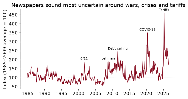
The most successful dictionary in economics is Baker, Bloom and Davis’s (2016) Economic Policy Uncertainty (EPU) index. The logic is a three-way filter. An article counts if it contains at least one term from each of three lists:
Each paper’s monthly count is divided by its total number of articles, standardised, averaged across ten major US newspapers, and scaled so that the index averaged 100 over 1985–2009. Requiring all three sets is what makes it precise: “uncertainty” alone catches sports and weather, “economy” alone catches everything. As regexes:
E = re.compile(r"\beconom(?:y|ic)\b", re.I)
P = re.compile(r"\b(?:congress|deficit|federal reserve|legislation|regulation|white house)\b", re.I)
U = re.compile(r"\buncertain(?:ty)?\b", re.I)
def is_epu(article):
    return all(rx.search(article) for rx in (E, P, U))
[is_epu(h) for h in ["Uncertainty over White House tariff plans weighs on the economy",
                     "Economic growth beats forecasts as consumers keep spending",
                     "Federal Reserve holds rates steady"]]
[True, False, False]
Only the first headline passes all three. We cannot run the filter on ten newspapers ourselves, but FRED publishes the result as series USEPUINDXM, and anyone can download it without a key:
The series runs from 1985 to September 2026. Its 1985–2009 average is 101.1, close to the 100 the construction promises (the published series has been revised since it was first scaled). It reached 190 in October 2008 and 350 during the 2020 pandemic, and its highest value so far, 460, came in April 2025, the month of the broad US tariff announcements.
Ten words, applied to millions of articles, gave macroeconomists a monthly measure of something they had theorised about for decades and never observed. Baker, Bloom and Davis then show that firms more exposed to government policy cut investment and hiring when the index rises. Just as important is how they validated it: research assistants read and coded thousands of articles by hand, and the dictionary index tracks the human one closely. A dictionary you have not checked against human judgement is a guess.
Suppose a newspaper changes its style guide and starts writing “the Fed” instead of “the Federal Reserve”. What happens to that paper’s contribution to the index, and how would you notice?
Articles about Fed policy uncertainty that used to pass the P filter now fail it, unless they also mention Congress, the deficit or another policy term, so the paper’s EPU count falls for reasons that have nothing to do with uncertainty. Because each paper is standardised separately, the drop shows up as a level shift in one paper’s series, starting on the date of the style change. You would notice it by plotting each newspaper’s series separately and looking for breaks that the other papers do not share. This is the general weakness of dictionaries: their validity rests on the words, and the words people use change over time even when the world does not.
If someone has already labelled some documents, you do not have to guess the dictionary. Let the labels choose it. Put the tf-idf matrix on the right-hand side of a regression (logistic for a category, linear for a number) and let the data decide which words predict the label.
| The obstacle is obvious to anyone who has run a regression. Text is high-dimensional: with unigrams and bigrams, our FOMC training sentences have thousands of columns and fewer than a thousand hawkish or dovish rows. OLS cannot even be computed when there are more columns than rows. Chapter 11 has the answer. The LASSO adds a penalty $\lambda \sum_j | \beta_j | $ to the loss, which sets most coefficients to exactly zero; cross-validation picks $\lambda$. In this setting the LASSO has a lovely interpretation: the words it keeps, with their signs, are a learned dictionary. |
Keep the hawkish and dovish sentences (dropping neutral gives a clean yes/no problem), and fit:
from sklearn.linear_model import LogisticRegressionCV
from sklearn.pipeline import make_pipeline
bin_tr, bin_te = train[train["label"] < 2], test[test["label"] < 2]    # 1 = hawkish, 0 = dovish
model = make_pipeline(
    TfidfVectorizer(ngram_range=(1, 2), min_df=2, sublinear_tf=True),
    LogisticRegressionCV(Cs=10, cv=5, penalty="l1", solver="liblinear",
                         scoring="accuracy", random_state=368))
model.fit(bin_tr["sentence"], bin_tr["label"]);
On the 249 held-out test sentences, the model is right 73.1% of the time, against 54.2% for always guessing the more common class. Cross-validation kept 188 of 5,599 features. Here are the ones with the largest weights:
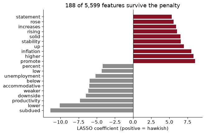
The hawkish side has promote, higher, inflation, up, stability, solid; the dovish side has subdued, lower, productivity, downside, weaker, accommodative. Much of that is central-bank vocabulary that an economist would have written down: inflation and higher on one side, subdued, lower, downside and accommodative on the other. Nobody told the model. Some of it is economics an economist might not have thought to write down: “productivity” leans dovish, presumably because faster productivity growth lets the economy grow without inflation, which argues for patience. And some of it no economist would choose, and those are the words to stare at. A word like “promote” probably reflects which documents happened to be sampled and labelled (speeches that “promote” price stability, say), not anything about the stance of policy. A learned dictionary is only as general as the sample that taught it.
Now the rental ads. Restrict to San Francisco, rents between $500 and $10,000, and known bedroom counts, which leaves 52,798 ads; split them 75/25. A colleague fits a LASSO of log rent on the tf-idf of the raw, lowercased titles and reports a test $R^2$ of 0.79. Is the text really that informative?
No. 87% of all titles contain a dollar figure, and we saw that it matches the rent almost perfectly. The model has learned to read “$2400” as a feature. It is the text version of Chapter 12’s reservation_status: a feature that contains the outcome. Exercise 22’s fix is to remove every dollar amount, every “Nbr” and every square-footage pattern anywhere in the title, not only in the prefix:
LEAK = r"\$\s?\d[\d,]*|\b\d+\s?br\b|\b\d+\s?ft(?:²|2)"
rent["text"] = (rent["title"].fillna("").map(html.unescape).str.lower()
                .str.replace(LEAK, " ", regex=True)
                .str.replace(r"\s+", " ", regex=True).str.strip(" -/"))
assert not rent["text"].str.contains(r"\$\d").any()
Refit on the cleaned titles, with the penalty chosen by three-fold cross-validation, and the test $R^2$ falls to 0.52. That is the honest number, and it is still respectable: words like “studio”, “room” and “furnished” really do tell you about a flat. The gap of 0.27 was the price itself.
The cleaned model keeps 1,522 of 5,038 features. Its largest positive and negative coefficients:
higher rent: resim, 图片, seasons, wavro, 3456, 3brm, 3ba, regis, sleek, paragon, rmdld view, skybox
lower rent:  studio, share, room available, remodeled pet, studios, law, room rent, neighbrs, bay area, francisco ca, roomate, efficiency
The negative side is mostly sensible: rooms, shares, studios, roommates. The positive side is a lesson in reading a learned dictionary. Some of it is informative (luxury buildings, garages, views). Some of it is leakage that my regex missed: “3brm” is a bedroom count written in a form the regex did not anticipate, and “3ba” and “4ba” are bathroom counts, which mark big flats; 9.0% of all the cleaned titles still contain a bathroom count. Some of it is a proxy for time: “resim” (Turkish for “picture”) and 图片 (Chinese for “picture”) are words that appeared in archived Craigslist pages in later years, when rents were higher, so the model uses them as a calendar. And some features are the names of realtors or buildings that post many listings, which identify a landlord rather than describe a flat.
None of these would show up in a test $R^2$. They all show up in five minutes of reading coefficients.
Everything in this chapter produces a $\hat V$ that is meant to go into something else: an index into a VAR, a stance score into an event study, a text-predicted rent into a housing study. So the usual econometric worries apply, with a twist. $\hat V$ is a generated regressor measured with error, and the errors are not always noise.
If the error is pure noise, unrelated to everything else, a $\hat V$ on the right-hand side biases its coefficient towards zero (attenuation), and a $\hat V$ on the left-hand side just widens your standard errors. That is the friendly case. The unfriendly case is error that is correlated with the thing you are studying. If the FOMC changed its vocabulary after 2008, and the classifier was trained mostly on pre-2008 sentences, then its errors are correlated with time, and any “change in stance after 2008” is partly a change in vocabulary. If a newspaper’s style guide changes, the EPU index jumps.
Three habits help. Validate against humans: hand-label a few hundred documents the model has not seen and report agreement, as Baker, Bloom and Davis did. Look at the errors, not just the accuracy: read the documents the model gets wrong, and check whether errors cluster by year, source or group. Report robustness to preprocessing: Denny and Spirling (2018) show that results can flip with choices as innocent-looking as stopword lists and stemming. Treat the pipeline the way you treat a set of control variables: show the result under a few reasonable alternatives.
You want to use the LASSO’s predictions to compare how hawkish the Fed sounded before and after 2008. Compare the model’s predicted hawkish share with the humans’ share in each period, on the test sentences.
                sentences  accuracy  human hawkish  predicted hawkish
era
2008 and after      133.0     0.729          0.436              0.481
before 2008         116.0     0.733          0.483              0.509
Read the last two columns as the measurement check. If the predicted and human shares move together across the two periods, the classifier preserves the comparison you care about, even though it misclassifies individual sentences. If accuracy differs a lot between the periods, the errors are correlated with time and your before-and-after comparison is partly an artefact. With only 116 to 133 test sentences per period, differences of a few percentage points are well within sampling noise (Chapter 8’s bootstrap would put a number on that), so the honest conclusion from a table like this is usually “no evidence of drift, and not much power to detect it”. That is worth saying out loud in a paper.
The two supervised pipelines from start to finish: the FOMC stance classifier and the rental-title regression.
import re, html
from pathlib import Path
import numpy as np, pandas as pd
from sklearn.feature_extraction.text import TfidfVectorizer
from sklearn.linear_model import LogisticRegressionCV, LassoCV
from sklearn.model_selection import train_test_split
from sklearn.pipeline import make_pipeline
from sklearn.metrics import accuracy_score, r2_score
SEED = 368
Load the FOMC sentences once and cache them; Shah, Paturi and Chava’s own train/test split is the one to use, so results are comparable with theirs.
HF = "https://huggingface.co/datasets/gtfintechlab/fomc_communication/resolve/main/"
def cached_csv(name, url):
    path = Path("../data") / name
    if not path.exists():
        pd.read_csv(url).to_csv(path, index=False)
    return pd.read_csv(path)
train, test = cached_csv("fomc_train.csv", HF + "train.csv"), cached_csv("fomc_test.csv", HF + "test.csv")
for df_ in (train, test):
    df_["stance"] = df_["label"].map({0: "dovish", 1: "hawkish", 2: "neutral"})
bin_tr, bin_te = train[train["label"] < 2], test[test["label"] < 2]
Fit the LASSO logistic regression on tf-idf, then score once on the test set.
stance = make_pipeline(TfidfVectorizer(ngram_range=(1, 2), min_df=2, sublinear_tf=True),
                       LogisticRegressionCV(Cs=10, cv=5, penalty="l1", solver="liblinear",
                                            scoring="accuracy", random_state=SEED))
stance.fit(bin_tr["sentence"], bin_tr["label"])
print(f"test accuracy {accuracy_score(bin_te['label'], stance.predict(bin_te['sentence'])):.3f}, "
      f"majority class {bin_te['label'].value_counts(normalize=True).max():.3f}")
test accuracy 0.731, majority class 0.542
The rental titles: clean out the leak, restrict to San Francisco, split.
rent = cached_csv("rent.csv", RENT_URL)
rent["log_price"] = np.log(rent["price"])
LEAK = r"\$\s?\d[\d,]*|\b\d+\s?br\b|\b\d+\s?ft(?:²|2)"
rent["text"] = (rent["title"].fillna("").map(html.unescape).str.lower()
                .str.replace(LEAK, " ", regex=True).str.replace(r"\s+", " ", regex=True).str.strip(" -/"))
sf = (rent.query("city == 'san francisco' and 500 <= price <= 10000")
          .dropna(subset=["beds"]).loc[lambda d: d["text"].str.len() > 0])
tr, te = train_test_split(sf, test_size=0.25, random_state=SEED)
Text alone, then structure alone (bedrooms, year and neighbourhood dummies), then both.
import scipy.sparse as sp
from sklearn.linear_model import LinearRegression, Lasso
tfv = TfidfVectorizer(min_df=10, ngram_range=(1, 2), sublinear_tf=True, stop_words="english")
T_tr, T_te = tfv.fit_transform(tr["text"]), tfv.transform(te["text"])
ybar = tr["log_price"].mean()
text_only = LassoCV(cv=3, alphas=np.logspace(-4.5, -2.5, 5), max_iter=3000).fit(T_tr, tr["log_price"] - ybar)
dummies = lambda d: pd.get_dummies(d[["nhood", "year"]].astype(str)).assign(beds=d["beds"]).astype(float)
S_tr = dummies(tr); S_te = dummies(te).reindex(columns=S_tr.columns, fill_value=0)
struct = LinearRegression().fit(S_tr, tr["log_price"])
both = Lasso(alpha=text_only.alpha_, max_iter=3000).fit(
    sp.hstack([T_tr, sp.csr_matrix(S_tr.values)]).tocsr(), tr["log_price"] - ybar)
r2 = {"text only": r2_score(te["log_price"], text_only.predict(T_te) + ybar),
      "structure only": r2_score(te["log_price"], struct.predict(S_te)),
      "text + structure": r2_score(te["log_price"],
                                   both.predict(sp.hstack([T_te, sp.csr_matrix(S_te.values)]).tocsr()) + ybar)}
pd.Series(r2).round(3)
text only           0.517
structure only      0.679
text + structure    0.772
dtype: float64
Bedrooms, neighbourhood and year explain 68% of the variance in log rent on the test ads; the cleaned title alone explains 52%; together they explain 77%. So the title adds 9 percentage points beyond the structured columns. Some of that is real information about the flat and some, as we saw, is bathrooms and calendar years sneaking in through the words. (One technical note: the “both” model reuses the penalty chosen for text alone and leaves the dummies unscaled, so it is a quick comparison, not a tuned model.)
Leaving the label in the text. 87% of rental titles contain the price, and a model trained on raw titles scores an $R^2$ of 0.79 by reading it. Ask of every text field what it records and when: a title written by the landlord after choosing the rent can contain the rent. The same goes for coders’ remarks in hand-labelled data, which Chapter 20 meets in the CEO departure notes.
Using a dictionary from another domain. A general-purpose list of negative words calls “liability”, “tax” and “crude” negative, which in a 10-K they are not. Either use a list built for your domain or validate a general one against human labels in your domain.
Measuring the wrong concept. Tone is not stance, and sentiment is not uncertainty. The net-tone dictionary separated hawkish from dovish sentences with an AUC of only 0.60, because “positive” is not a monetary-policy concept. Name $V$ first and choose the method second.
Ignoring negation and context. “Inflation has not declined” counts as a negative-tone sentence. Bigrams help a little, and the contextual models of Chapter 21 help a lot, but a bag of words will never read a sentence.
Trusting a learned dictionary without reading it. The rental LASSO kept bathroom counts, foreign words for “picture” and realtor names. None of these show up in an $R^2$. Print the coefficients, and for any surprising word, read five documents that contain it.
Tuning the pipeline on the test set. There are dozens of preprocessing choices (case, stopwords, stemming, n-grams, min_df), and trying them all and reporting the best test score is the text version of specification searching. Choose them by cross-validation on training data, or fix them in advance, and report a few alternatives.
The EPU filter requires an article to contain a term from each of the E, P and U lists. Explain what would go wrong with an index that counted articles containing just “uncertain” or “uncertainty”. What would go wrong if it required only E and U?
Loughran and McDonald found that words like “liability” and “cost” are not negative in 10-Ks. Give an example of a word that would be misclassified by a general-purpose sentiment dictionary in FOMC text, and explain why.
Using the illustrative lm word lists, compute the share of FOMC training sentences of each stance (hawkish, dovish, neutral) that contain at least one uncertainty word. Do neutral sentences sound more uncertain than the others?
Fit the LASSO logistic regression on all three classes (dovish, hawkish, neutral) using the same tf-idf settings. Report test accuracy and compare it with the majority-class baseline. Is the gain over the baseline larger or smaller than in the two-class problem?
Preprocessing robustness: refit the two-class FOMC model with unigrams only (ngram_range=(1, 1)), and separately with min_df=5. Report the test accuracy of each next to the original. What would you write in a paper’s robustness section?
Extend the leak regex to also remove bathroom counts such as “2ba” or “1.5ba”. What share of the cleaned San Francisco titles contained one? Refit the text-only LASSO with the chosen penalty and report the change in test $R^2$.
A city housing office wants to use the text model to flag “overpriced” listings: ads whose rent is far above the model’s prediction. What would you need to show them first? Think about leakage, time and what the residual measures.
1. “Uncertain” alone catches every article about uncertain weather, uncertain playoffs and uncertain elections, so the index would mostly measure the volume of news, not policy uncertainty. Requiring E and U but not P catches uncertainty about the economy for any reason (a hurricane, an oil shock, a bank failure), which is economic uncertainty in general rather than uncertainty about policy. The three-way filter is what makes the index specific to the concept in its name, and the human audit is how Baker, Bloom and Davis checked that it is.
2. One example is “unemployment”, which a general dictionary might treat as negative. In FOMC text the word appears in hawkish sentences (“the unemployment rate has declined to a low level”) and dovish ones (“unemployment remains elevated”) alike, because it is the name of one half of the Fed’s mandate. Another is “accommodation” or “accommodative”: neutral or even warm in ordinary English, but a technical term for easy policy. A domain changes what words mean.
3.
unc = train.assign(any_unc=[any(t in lm["uncertainty"] for t in tokens(s)) for s in train["sentence"]])
unc_share = unc.groupby("stance")["any_unc"].mean()
print(unc_share.round(3).to_string())
stance
dovish     0.188
hawkish    0.189
neutral    0.165
19% of dovish, 19% of hawkish and 16% of neutral sentences contain an uncertainty word. The three shares are within 2 percentage points of each other, so no: by this measure neutral sentences do not sound more uncertain than the others, and uncertainty words tell you almost nothing about stance. Note how blunt the instrument is: “may” and “could” are on the list, and they are as much grammar as doubt. A real test would use the full Loughran–McDonald uncertainty list and check a sample of sentences by hand.
4.
from sklearn.multiclass import OneVsRestClassifier     # liblinear fits two classes at a time
three = make_pipeline(TfidfVectorizer(ngram_range=(1, 2), min_df=2, sublinear_tf=True),
                      OneVsRestClassifier(LogisticRegressionCV(Cs=10, cv=5, penalty="l1", solver="liblinear",
                                                               scoring="accuracy", random_state=SEED)))
three.fit(train["sentence"], train["label"])
acc3 = accuracy_score(test["label"], three.predict(test["sentence"]))
base3 = test["label"].value_counts(normalize=True).max()
print(round(acc3, 3), round(base3, 3))
0.609 0.498
Three-class accuracy is 60.9% against a baseline of 49.8% (always “neutral”). The gain is 11 percentage points, against 19 in the two-class problem. Smaller: neutral is the hardest class to pin down with words, because a neutral sentence is defined by what it does not say.
5.
def acc_with(**kw):
    m = make_pipeline(TfidfVectorizer(sublinear_tf=True, **kw),
                      LogisticRegressionCV(Cs=10, cv=5, penalty="l1", solver="liblinear",
                                           scoring="accuracy", random_state=SEED))
    return accuracy_score(bin_te["label"], m.fit(bin_tr["sentence"], bin_tr["label"]).predict(bin_te["sentence"]))
rob = {"original (1-2 grams, min_df=2)": acc_lasso,
       "unigrams only": acc_with(ngram_range=(1, 1), min_df=2),
       "min_df=5": acc_with(ngram_range=(1, 2), min_df=5)}
print(pd.Series(rob).round(3).to_string())
original (1-2 grams, min_df=2)    0.731
unigrams only                     0.759
min_df=5                          0.731
The three accuracies are 73.1%, 75.9%, 73.1%. With 249 test sentences, one sentence is 0.4% of accuracy, so the largest gap, 2.8 points, is about 7 sentences. A paper would report the whole table and say that performance moves by a few sentences across reasonable pipelines, which is within sampling noise. What it must not do is pick the best-looking variant because it scored best on the test set: that turns the test set into a training set, and the reported accuracy would be optimistic.
6.
BA = r"\b\d(?:\.\d)?\s?ba\b"
share_ba = sf["text"].str.contains(BA).mean()
tr2, te2 = tr["text"].str.replace(BA, " ", regex=True), te["text"].str.replace(BA, " ", regex=True)
v2 = TfidfVectorizer(min_df=10, ngram_range=(1, 2), sublinear_tf=True, stop_words="english")
m2 = Lasso(alpha=text_only.alpha_, max_iter=3000).fit(v2.fit_transform(tr2), tr["log_price"] - ybar)
r2_noba = r2_score(te["log_price"], m2.predict(v2.transform(te2)) + ybar)
print(round(share_ba, 3), round(r2_text, 3), round(r2_noba, 3))
0.1 0.517 0.509
10.0% of cleaned San Francisco titles contained a bathroom count. Removing them moves the text-only test $R^2$ from 0.517 to 0.509. Whether that is “leakage” is a judgement: the number of bathrooms is a genuine feature of the flat, and a housing office would know it. The problem is only that it is not what we meant by “what the words add”. If you want to measure that, put bathrooms in the structured model and take them out of the text.
7. At least four things. First, that the model contains no leak: no prices, and ideally no bedroom or bathroom counts in the text, which belong in the structured part. Second, that it predicts well on listings from a later period than it was trained on (a time split, as in Chapter 12’s exercise), since rents and Craigslist’s page format both changed over the years and words like “resim” are calendar proxies. Third, what the residual actually measures: a listing is “overpriced” relative to the model only if the model sees everything that justifies a high rent, and a one-line title does not mention the renovated kitchen. A large residual is as likely to be an unmeasured amenity as an overcharge. Fourth, who would be flagged: if residuals are systematically larger in some neighbourhoods or for some kinds of landlord, the tool would target them, and the office should see the error rates by group before using it.
Gentzkow, Matthew, Bryan Kelly and Matt Taddy (2019). “Text as Data.” Journal of Economic Literature 57(3): 535–574. doi.org/10.1257/jel.20181020
The survey that gave this chapter its framework. The authors set out the represent, measure, use pipeline, explain why text is a high-dimensional problem, and walk through dictionaries, penalised regressions, topic models and word embeddings with examples from finance, macroeconomics and political economy. The early sections are readable with nothing more than this chapter and Chapter 11.
Think about: the authors stress that $\hat V$ is usually an input to a second-stage economic analysis. If the errors in $\hat V$ are correlated with your treatment variable, what happens to your estimate, and which of this chapter’s validation habits would detect it?
Baker, Scott R., Nicholas Bloom and Steven J. Davis (2016). “Measuring Economic Policy Uncertainty.” Quarterly Journal of Economics 131(4): 1593–1636. doi.org/10.1093/qje/qjw024
The paper behind the EPU index. Baker, Bloom and Davis build the index from three short word lists applied to ten US newspapers, validate it against a large human audit of articles, and extend it to other countries and to specific policy areas. They then show that firms more exposed to government purchases cut investment and employment when policy uncertainty rises, and that at the aggregate level spikes in the index foreshadow declines in investment, output and employment.
Think about: the index rises when newspapers write more about policy uncertainty. Can you think of a reason newspapers might write more about uncertainty when the economy is already weakening for other reasons? What would that do to the paper’s claim that uncertainty causes firms to cut investment?
Shah, Agam, Suvan Paturi and Sudheer Chava (2023). “Trillion Dollar Words: A New Financial Dataset, Task & Market Analysis.” Proceedings of the 61st Annual Meeting of the Association for Computational Linguistics (Volume 1: Long Papers): 6664–6679. doi.org/10.18653/v1/2023.acl-long.368
The source of our FOMC sentences. The authors collect FOMC statements, minutes and speeches, have them labelled hawkish, dovish or neutral, and compare classifiers from simple word-count models up to large language models on the task. They then aggregate sentence-level predictions into a monthly stance measure and relate it to inflation and market data. It is a computer-science conference paper, so expect less economics and more benchmarking than in a journal article.
Think about: the Fed chooses its words knowing that markets parse them. If the Committee learns that certain words move markets, it may stop using them. What does that strategic behaviour do to a learned dictionary trained on older statements, and to the comparison of stance across decades?
Reading. Gentzkow, Kelly & Taddy (2019), sections 1–3, for the framework. Loughran & McDonald (2011), “When Is a Liability Not a Liability? Textual Analysis, Dictionaries, and 10-Ks”, Journal of Finance 66(1), for why domain matters. Denny & Spirling (2018), “Text Preprocessing for Unsupervised Learning”, Political Analysis, for how preprocessing choices change results. Grimmer, Roberts & Stewart (2022), Text as Data, Princeton University Press, for a book-length treatment. Jurafsky & Martin, Speech and Language Processing (3rd ed. draft, free online), ch. 2, for regular expressions and tokenization.