The question: a language model can label ten thousand Fed sentences as hawkish or dovish in an afternoon, for less than the cost of one research assistant’s lunch. Should an economist trust those labels, and what exactly is the machine that produced them trying to do?
Chapters 19 and 20 represented text in two ways: as a bag of word counts, and as embedding vectors. Both have blind spots that matter for economics.
A bag of words ignores order, so “inflation rose and unemployment fell” and “unemployment rose and inflation fell” are the same document. It ignores negation, so “not hawkish” contains the word “hawkish”. And word2vec gives each word one vector whatever the sentence, so the “ease” in “the Fed will ease policy” and the “eased” in “inflation pressures eased” are treated alike, though one is a policy action and the other a price movement. “Bank” gets one vector for a river bank and a central bank.
A transformer (Vaswani and coauthors, 2017) fixes this by building a different vector for each word in each sentence, letting every word look at every other word before deciding what it means. The mechanism is called attention, and it is the core of every modern language model, from BERT to the chat assistants. This chapter explains attention and tokenization at the level you need to use these models sensibly, shows how to use them from Python, explains how the chat models are trained to behave the way they do, and spends most of its time on the economist’s question: when a model labels your data, how do you know the labels are any good?
Start with one vector per token, the kind of embedding Chapter 20 learned. Attention asks, for each token, which other tokens should I borrow information from? Each token’s vector $\mathbf{x}_i$ is multiplied by three learned matrices to produce three new vectors:
Token $i$ compares its query with every key by a dot product. A large dot product means “this is the kind of token I am looking for”. The scores are turned into weights that sum to one with the softmax function (the multinomial logit formula from econometrics), and the new vector for token $i$ is the weighted average of the values:
\[\text{new}_i = \sum_j w_{ij}\,\mathbf{v}_j, \qquad w_{ij} = \frac{e^{\mathbf{q}_i \cdot \mathbf{k}_j / \sqrt d}}{\sum_m e^{\mathbf{q}_i \cdot \mathbf{k}_m / \sqrt d}}.\]Dividing by $\sqrt d$, the square root of the vector length, keeps the scores from getting so large that the softmax puts all its weight on one token. That is the whole of attention. In code:
rng = np.random.default_rng(368)
tokens = ["the", "fed", "will", "ease", "policy"]
d = 8
X = rng.normal(size=(len(tokens), d))                          # one (toy) embedding per token
W_Q, W_K, W_V = (rng.normal(size=(d, d)) / np.sqrt(d) for _ in range(3))
Q, K, V = X @ W_Q, X @ W_K, X @ W_V
A = softmax(Q @ K.T / np.sqrt(d))                              # 5 x 5 attention weights
H = A @ V                                                      # one new vector per token
print(pd.DataFrame(A, index=tokens, columns=tokens).round(2))
         the   fed  will  ease  policy
the     0.10  0.02  0.06  0.19    0.62
fed     0.14  0.42  0.29  0.08    0.07
will    0.05  0.08  0.10  0.30    0.46
ease    0.17  0.70  0.05  0.06    0.02
policy  0.12  0.06  0.04  0.54    0.24
Row $i$ is how much token $i$ attends to each token, and each row sums to one. Here the matrices are random, so the pattern means nothing. In a trained model they are learned from billions of sentences, so that, for example, “ease” learns to attend to “fed” and “policy” and comes out with a vector that means monetary easing, while the “eased” in a sentence about prices attends to “inflation” and comes out meaning something else. Same word, different vector: that is a contextual embedding.
A real transformer runs many attention calculations in parallel (multi-head attention, each head free to specialise in something like grammar or negation), passes the result through a small neural network, and stacks this block a dozen to a hundred times. Because attention on its own ignores order, a positional encoding is added to each token’s vector so the model knows which word came first. Everything is matrix multiplication, which is why transformers can be trained on enormous amounts of text with graphics processors: they scale.
A hypothetical sentence has two tokens, “not” and “hawkish”. The query for “hawkish” has dot products of 2 with the key of “not” and 0 with its own key, and $d = 4$. The values are $\mathbf{v}{\text{not}} = (1, 0)$ and $\mathbf{v}{\text{hawkish}} = (0, 1)$. What is the new vector for “hawkish”?
Divide the scores by $\sqrt 4 = 2$ to get $(1, 0)$, and take the softmax: $e^1/(e^1 + e^0) =$ 0.731 on “not” and 0.269 on itself. The new vector is 0.731 × (1, 0) + 0.269 × (0, 1) = (0.73, 0.27). Most of the new “hawkish” vector now comes from “not”. That is how a transformer can represent “not hawkish” as something different from “hawkish”, which no bag of words can do.
Transformers do not see words. They see tokens from a fixed vocabulary, typically 30,000 to 200,000 pieces, and a rare word is split into several pieces. The most common way of building that vocabulary is byte-pair encoding (BPE). Start with single characters. Count every pair of adjacent symbols in a training corpus, merge the most frequent pair into a new symbol, and repeat, thousands of times. Frequent words end up as single tokens; rare words are spelled out from frequent pieces, so the model never meets a word it cannot represent.
Here is BPE on a tiny made-up corpus of economics words, with how often each appears:
def bpe(word_counts, n_merges):
    vocab = {tuple(w): c for w, c in word_counts.items()}       # each word as a tuple of symbols
    merges = []
    for _ in range(n_merges):
        pairs = Counter()
        for sym, c in vocab.items():
            for a, b in zip(sym, sym[1:]):
                pairs[a, b] += c
        (a, b), _ = pairs.most_common(1)[0]                      # the most frequent adjacent pair
        merges.append(a + b)
        vocab = {tuple(re.sub(rf"(?<!\S){re.escape(a)} {re.escape(b)}(?!\S)", a + b,
                              " ".join(sym)).split()): c for sym, c in vocab.items()}
    return merges, vocab
corpus = {"inflation": 10, "deflation": 4, "stagflation": 2, "nation": 3, "inflationary": 3}
merges, vocab = bpe(corpus, 8)
print(merges); print(list(vocab))
['at', 'ati', 'atio', 'ation', 'fl', 'flation', 'in', 'inflation']
[('inflation',), ('d', 'e', 'flation'), ('s', 't', 'a', 'g', 'flation'), ('n', 'ation'), ('inflation', 'a', 'r', 'y')]
After eight merges, the common ending “flation” is a single piece, so a word the corpus never contained, such as “reflation”, could be written with just two or three tokens. Real tokenizers do the same on terabytes of text.
Two real tokenizers on one Fed sentence: BERT’s (WordPiece, a close cousin of BPE, which marks continuation pieces with ##) and GPT-2’s (byte-level BPE, which marks a leading space with Ġ):
for name, tok in [("bert-base-uncased", tok_bert), ("gpt2", tok_gpt2)]:
    print(f"{name:18s}", tok.tokenize(s_tok))
bert-base-uncased  ['quantitative', 'tightening', 'sh', '##rank', 'the', 'f', '##om', '##c', "'", 's', 'balance', 'sheet', 'unexpectedly', '.']
gpt2               ['Quant', 'itative', 'Ġtightening', 'Ġshr', 'ank', 'Ġthe', 'ĠF', 'OM', 'C', "'s", 'Ġbalance', 'Ġsheet', 'Ġunexpectedly', '.']
“FOMC” is not in either vocabulary, so both split it. Tokenization matters to an economist for three practical reasons. Cost: commercial models bill per token, and across the 496 FOMC test sentences GPT-2’s tokenizer produces 1.18 tokens per word. Context limits are measured in tokens: BERT reads at most 512. And numbers are split into arbitrary pieces (“3.75” may be several tokens), which is one reason language models can be unreliable at arithmetic.
You want an LLM to label 100,000 FOMC sentences. Each request carries about 250 input tokens (instructions plus one sentence) and returns about 60 output tokens. At $2 per million input tokens and $10 per million output tokens, roughly the list price of a mid-tier model such as Claude Sonnet 5.5 when this was written (check the current price list before budgeting), what does it cost?
Input: $100{,}000 \times 250 = 25$ million tokens, at $2 per million, is $50. Output: $100{,}000 \times 60 = 6$ million tokens, at $10 per million, is $60. The total is $110. The major providers offer a batch interface for jobs that can wait a day at about half price, so roughly $55. Two lessons. First, this is very cheap compared with human labelling, which is why the method has spread so fast. Second, the instructions dominate the input bill: a 250-token request built around an FOMC sentence of about 35 tokens means you pay mostly for repeating yourself, and a longer codebook with worked examples (which usually improves accuracy) multiplies the cost.
Language models are trained in two stages, and the distinction is the most useful idea in this chapter.
Pretraining is expensive and done once, by a company or a lab. The model reads billions of words of ordinary text and learns to predict missing words. No one labels anything: the text is its own label. To get good at predicting words, the model has to learn grammar, facts, and a great deal about how the world fits together.
Fine-tuning (or adaptation) is cheap and done by you. Take the pretrained model and train it a little more on a small labelled dataset for your task. Most of the knowledge comes from pretraining; your few thousand labelled FOMC sentences only have to teach the last mile. Econometricians will recognise the logic of using a first stage estimated elsewhere. The name in machine learning is transfer learning.
The two families of transformer differ in their pretraining task.
| BERT (encoder) | GPT (decoder) | |
|---|---|---|
| Pretraining task | fill in a masked word | predict the next word |
| Context it sees | both directions | only the words before |
| Good at | understanding: classification, embeddings | generating: writing, chat, reasoning |
| Typical use in research | fine-tune a classifier | prompt it, or fine-tune |
Here is BERT’s pretraining task in action, with a small version of BERT. Nobody labelled anything; it learned this by filling in blanks in books and Wikipedia:
for s, top in fill_out.items():
    print(s, "->", [(r["token_str"], round(r["score"], 2)) for r in top])
The Federal Reserve raised interest [MASK] to fight inflation. -> [('rates', 0.77), ('funds', 0.05), ('payments', 0.03)]
Unemployment [MASK] sharply in April 2020. -> [('fell', 0.3), ('declined', 0.28), ('rose', 0.1)]
It knows that the Fed raises rates. And it guesses that unemployment fell sharply in April 2020, when in fact the US unemployment rate jumped from 4.4% in March to 14.8% in April (FRED series UNRATE). DistilBERT’s training text predates the pandemic, so it has no way of knowing; it can only guess what usually follows “unemployment” in the text it read. A model knows only what was in its training data, up to the date the data end. Hold on to that: it is the root of the look-ahead problem later in the chapter.
For each task, would you reach for a BERT-style encoder or a GPT-style decoder? (a) Scoring 2 million earnings-call sentences for sentiment, with 5,000 hand-labelled ones available. (b) Writing a one-paragraph summary of each of 300 FOMC minutes. (c) Labelling 500 CEO departure notes when you have no labelled examples at all.
(a) An encoder, fine-tuned on the 5,000 labels. It is small, fast and cheap enough to run on 2 million sentences, and with that many labels fine-tuning usually beats prompting. (b) A decoder: summarising is generation. (c) Either a zero-shot classifier (an encoder trained for a related task, next section) or a prompted decoder. With no labels, prompting is the only option. But you still need some labels, a couple of hundred coded by hand, to check the output. That is the theme of the rest of the chapter.
The transformers library from Hugging Face wraps a model and its tokenizer in a pipeline: one line downloads the model, and one line uses it. The course environment has the models this chapter needs cached locally.
A general sentiment model, trained on movie reviews, applied to Fed sentences:
sst = pipeline("sentiment-analysis", model="distilbert/distilbert-base-uncased-finetuned-sst-2-english")
print(pd.DataFrame(sst(fomc4)).assign(text=[s[:60] for s in fomc4]).round(3).to_string(index=False))
   label  score                                                         text
NEGATIVE  0.990 Job gains have been solid and the unemployment rate has rema
NEGATIVE  0.998    Inflation has not declined; the outlook is not favorable.
NEGATIVE  0.957 The Committee decided to raise the target range for the fede
POSITIVE  0.910                   Further policy firming may be appropriate.
It is confident, and it is answering the wrong question. “Positive” and “negative” are not monetary-policy concepts: a rate rise is bad news for bond holders and good news for the Fed’s inflation goal. Sentiment is not stance, exactly as tone was not stance in Chapter 19. Choose a model whose labels match your economic concept.
A zero-shot classifier lets you choose the labels. It is built from a model trained on natural-language inference: given a premise and a hypothesis, does the premise imply the hypothesis? Turn each label into a hypothesis (“The monetary policy stance of this text is hawkish”) and the model scores how strongly the sentence implies each one. No training data needed. The model the course uses is MoritzLaurer/deberta-v3-base-zeroshot-v2.0:
zsc = pipeline("zero-shot-classification", model="MoritzLaurer/deberta-v3-base-zeroshot-v2.0")
r = zsc("Further policy firming may be appropriate to bring inflation down.",
        candidate_labels=["hawkish", "dovish", "neutral"],
        hypothesis_template="The monetary policy stance of this text is {}.")
{lab: round(float(sc), 3) for lab, sc in zip(r["labels"], r["scores"])}
{'hawkish': 0.997, 'neutral': 0.002, 'dovish': 0.001}
That one looks right. One example proves nothing, which brings us to validation, but first a detour that matters for every chat model you will use.
A pretrained model does one thing: it predicts text. It has no goals, no notion of a question or an answer, and no values. Ask the pretrained DistilBERT model from the last section a question, leaving the answer as the blank it is trained to fill, and it does not answer; it predicts what kind of symbol usually comes next:
print(prompt_)
print([(r["token_str"], round(r["score"], 2)) for r in fill(prompt_)[:5]])
Question: is the sentence "The Committee will raise rates" hawkish or dovish? Answer: [MASK]
[('?', 0.31), ('!', 0.08), ('.', 0.06), ('…', 0.04), ('|', 0.04)]
Its top guesses are “?”, “!”, “.”. Neither “hawkish” nor “dovish” is anywhere near the top: after “Answer:” in ordinary text, punctuation is a better bet than an answer. A text predictor, however large, will continue a request for help with a crime as readily as a request for help with homework, and it will happily continue a falsehood. Usefulness, and restraint, have to be trained in.
The chat assistants you use are the same kind of model after further training that turns a text predictor into something that answers questions, follows instructions, and declines some requests. Roughly, there are three steps.
That third step is Constitutional AI (Bai and coauthors, 2022, arXiv:2212.08073), developed at Anthropic. A constitution is a written statement of the values and priorities the model should follow. Training happens in two phases. In the supervised phase, the model drafts a response, then is asked to critique its own draft against a principle from the constitution and revise it; the model is then fine-tuned on the revised responses. In the reinforcement-learning phase, the model compares pairs of its own responses and judges which better follows the constitution; those AI judgements train a preference model, which serves as the reward for reinforcement learning. Because the feedback comes from an AI applying written principles rather than from a person judging each pair, this is called reinforcement learning from AI feedback (RLAIF). The appeal is that the standards are explicit, can be published and argued about, and need far fewer human labels.
Anthropic has published the constitution it uses to train its Claude models (at anthropic.com/constitution, released under a CC0 public-domain dedication). It names four core properties and says how to rank them when they conflict. In order:
The document says the model should prioritise these “in the order in which they are listed” when they conflict, and it describes that prioritisation as holistic rather than a strict lexical ordering. It also stresses that in the vast majority of everyday tasks, such as coding, writing and analysis, the four do not conflict at all. The ordering is for the rare cases where they do.
The most common misconception is about when the constitution is used. The model does not look the constitution up when it answers you. There is no document consulted at answer time. The constitution shapes the training data and the feedback, and the values end up encoded in the model’s weights, the same billions of numbers that encode its grammar. It is closer to a professional’s training than to a rulebook on the desk.
On top of the trained values sit two more layers, and it helps to think of them as a chain of principals and agents:
| Layer | Who writes it | When it acts | Example |
|---|---|---|---|
| Constitution and training | the model’s developer | before release, in the weights | rank safety and ethics above helpfulness |
| System prompt | the business deploying the model (the “operator”) | at the start of every conversation | “You are a monetary-policy coding assistant. Answer only with a label.” |
| User message | the person using the product | each turn | “Label this sentence: …” |
Each layer works within the limits set by the one above. Claude’s constitution uses an analogy an economist will like: the operator is like a business owner who has taken on a worker from a staffing agency, where the agency has its own norms of conduct that take precedence over the business owner’s instructions. The business can direct the work without explaining every instruction; it cannot direct the worker to break the agency’s rules.
You use a chat model to label 5,000 FOMC sentences. Your instructions go in the system prompt. Name two ways the model’s training, rather than your prompt, could affect your labels.
First, helpfulness training can create a pull towards agreeing with the person asking. If your prompt hints at what you expect (“most of these sentences are hawkish”), a model trained on human preferences may drift towards confirming it, a tendency known as sycophancy. Write neutral instructions and keep your hypotheses out of the prompt. Second, the training is not yours to inspect and can change. When the developer releases a new version, trained with different data or feedback, the same prompt can produce different labels. Your measurement instrument has been recalibrated without notice. That is why you pin the exact model version, record it, and keep every response, as the next section explains. (A third, rarer effect: a model trained to decline some requests may refuse or hedge on unusual text. For FOMC sentences this almost never happens, but check for refusals rather than assume.)
Korinek (2023) catalogues how economists can use large language models across the research process: brainstorming, editing, summarising literature (verify every citation), writing and debugging code, and, the use that matters most for data work, classifying, extracting and scoring text at scale. In that last role the model is a measurement instrument: a research assistant who can read 100,000 documents. Like any instrument it must be calibrated against a standard, and the standard is human judgement.
Here is what labelling with an API looks like, using Anthropic’s Python SDK and the course’s codebook-style prompt. The code is shown, not run in this book: it needs an API key and costs money. The key is read from the ANTHROPIC_API_KEY environment variable; never paste a key into a notebook or commit it to GitHub.
import anthropic
from typing import Literal
from pydantic import BaseModel

client = anthropic.Anthropic()          # reads ANTHROPIC_API_KEY from the environment

class Stance(BaseModel):
    label: Literal["hawkish", "dovish", "neutral"]
    rationale: str                      # short; for auditing errors, not for scoring

SYSTEM = """You are an expert on U.S. monetary policy. Classify the stance of one sentence
from FOMC communications. hawkish = favours tighter policy or signals concern about inflation;
dovish = favours easier policy or signals economic weakness or slack; neutral = neither."""

def label_sentence(text):
    resp = client.messages.parse(
        model="claude-sonnet-5-5",      # pin the exact model ID and record it
        max_tokens=512,
        output_config={"effort": "low"},
        system=SYSTEM,
        messages=[{"role": "user", "content": f"Sentence: {text}"}],
        output_format=Stance,           # structured output, validated against the schema
    )
    return resp.parsed_output

# sample = test.sample(200, random_state=368)
# sample["llm"] = [label_sentence(s).label for s in sample["sentence"]]   # cache to disk!
Four habits are visible in that code. The codebook in the system prompt defines the construct as you would for a human research assistant. The structured output forces one of three labels rather than free text you would have to parse. The rationale is for reading errors, not for scoring. And the exact model ID is in the code, so you can report it.
We do not need an API key to practise validation, because the zero-shot classifier is a machine labeller too, and it runs locally. Label all 496 held-out FOMC test sentences from Shah, Paturi and Chava (2023), the same sentences as in Chapter 19, and compare with the human labels:
out = zsc(test["sentence"].tolist(), candidate_labels=["hawkish", "dovish", "neutral"],
          hypothesis_template="The monetary policy stance of this text is {}.", batch_size=16)
test["zeroshot"] = [o["labels"][0] for o in out]
print(f"accuracy {accuracy_score(test['human'], test['zeroshot']):.3f}, "
      f"kappa {cohen_kappa_score(test['human'], test['zeroshot']):.3f}")
accuracy 0.593, kappa 0.330
Accuracy is 59.3%. On its own that number is hard to read, because the classes are unbalanced: always guessing the most common human label, “neutral”, would score 49.8%. Cohen’s kappa corrects accuracy for the agreement you would get by chance:
\[\kappa = \frac{p_o - p_e}{1 - p_e},\]where $p_o$ is the observed share of agreement and $p_e$ is the agreement expected if the machine and the humans each assigned labels at random with their own frequencies. Kappa is 0 for chance agreement and 1 for perfect agreement. A rough and much-quoted scale (Landis and Koch, 1977) calls 0.21–0.40 “fair”, 0.41–0.60 “moderate” and 0.61–0.80 “substantial”. Here $\kappa =$ 0.33.
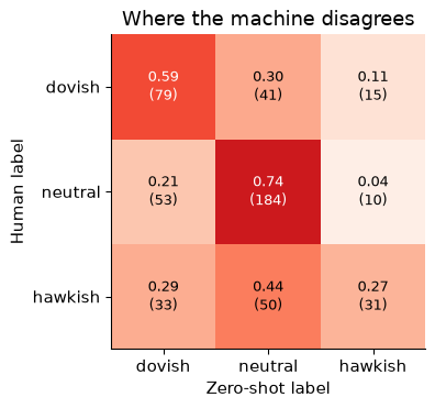
The confusion matrix shows where the disagreement is:
The model does best on neutral sentences and worst on hawkish ones: only 27% of the sentences humans called hawkish get that label. The pattern of errors matters more than the headline number. If you built a monthly “stance index” from these labels, a model that rarely recognises hawkish sentences would make the Fed look less hawkish than it was, and the bias would be worst in the years when the Fed was most hawkish. That is measurement error correlated with the thing you are measuring, the unfriendly kind from Chapter 19.
From the confusion matrix, compute $p_o$, $p_e$ and $\kappa$ and check against scikit-learn.
zeroshot  dovish  neutral  hawkish
human
dovish        79       41       15
neutral       53      184       10
hawkish       33       50       31
$p_o$ is the diagonal over the total: 294 / 496 = 0.593. For $p_e$, multiply the humans’ share of each label by the machine’s share of the same label and add up across the three labels: 0.393. Then κ = (0.593 − 0.393) / (1 − 0.393) = 0.330, matching scikit-learn’s 0.330. Notice that $p_e$ is not one third: chance agreement is high when both raters use “neutral” a lot, and kappa gives no credit for that.
Kappa of 0.33 for a model that has never seen a labelled FOMC sentence is not nothing. Is it good enough? Two comparisons help.
The first is a cheap supervised model. Freeze Chapter 20’s sentence encoder, embed the 1,984 labelled training sentences, and fit a logistic regression on top. On the same test sentences it scores accuracy 61.3% and kappa 0.36. Shah, Paturi and Chava report that a fully fine-tuned large encoder does better still. With a couple of thousand labels, training on them usually beats prompting.
The second is human agreement. Two trained economists labelling the same sentences do not agree perfectly either: hawkish and dovish are judgements. A machine that agrees with one human as well as a second human does is doing a research assistant’s job, and that, not 100%, is the benchmark. Gilardi, Alizadeh and Kubli (2023) ran exactly this comparison for several political-science annotation tasks and found that a chat model agreed with trained annotators more often than crowd workers did, at a fraction of the cost. A careful validation protocol therefore looks like this:
Step 3 is where people cheat without meaning to. Trying ten prompts and reporting the one that scored best on the validation set is tuning on the test set, exactly as in Chapter 9.
Cost is per token and falls every year; the worked example above is the calculation to do before you start. Batch interfaces halve it for work that can wait.
Reproducibility is harder than it looks. Providers retire models, and the same model can give different answers to the same prompt on different runs. Record the exact model ID, the prompt, the schema, the date and any settings; save every response to disk and label each document once; and report all of it in an appendix. Open-weight models that you download and run yourself, like the zero-shot classifier in this chapter, give you complete control of the version, which is a real advantage for research that must be replicated.
Look-ahead bias is the econometric problem specific to these models. A model trained on text up to some date has read what happened next. Ask it whether a 2007 earnings call predicts the firm’s returns and you are asking someone who has read about 2008. DistilBERT’s guess about April 2020 showed the other side of the same coin: a model knows what was in its training data and nothing after. Glasserman and Lin (2023) document look-ahead effects in return prediction from news, and Ludwig, Mullainathan and Rambachan (2025) set out when LLM-based measurement can and cannot support valid inference. The fixes: evaluate forecasts only on periods after the model’s training cutoff; mask firm names, people and dates so the model cannot recognise the event; prefer measurement tasks (is this sentence hawkish?) to forecasting tasks whose outcomes are in the training data.
Memorisation is the cousin of look-ahead. These FOMC sentences, and the press coverage of famous CEO departures, are public and may be in a large model’s training data. A model might label a note “fired” because it remembers the CEO, not because of what the note says. Masking names and comparing labels with and without them is the test.
Ethics. Do not send confidential or identifiable data (survey microdata, administrative records, student records) to an external API without approval from your institution and the data owner. Respect the terms of service and copyright of the text you feed in. Disclose how you used AI tools; journals increasingly require it. And remember that you, not the model, are responsible for every number in your paper. A hallucinated citation or a mislabelled variable is your error.
A researcher wants to show that an LLM’s reading of FOMC minutes predicts the next Treasury yield movement better than economists’ forecasts did, using minutes from 2000 to 2015. What is wrong, and how would you redesign the study?
The model was almost certainly trained on text written after 2015, including commentary on what yields did after each meeting. Its “prediction” may be memory. A redesign: (1) restrict the evaluation to minutes released after the model’s documented training cutoff; (2) or use a model trained only on text up to each date (some research groups now build such time-stamped models); (3) or turn the task from forecasting into measurement: have the LLM score only the stance of each sentence, validate those scores against human labels, and then estimate the relationship between stance and yields yourself, in a regression where look-ahead cannot enter. The third design is the safest, because the model is never asked a question whose answer it could have read.
The full validation exercise, runnable top to bottom with models cached locally: tokenize, label with the zero-shot classifier, compare with human labels and with a frozen-embedding classifier.
import numpy as np, pandas as pd
from pathlib import Path
from transformers import AutoTokenizer, pipeline
from sentence_transformers import SentenceTransformer
from sklearn.linear_model import LogisticRegression
from sklearn.metrics import accuracy_score, cohen_kappa_score, confusion_matrix
SEED = 368
HF = "https://huggingface.co/datasets/gtfintechlab/fomc_communication/resolve/main/"
train, test = cached_csv("fomc_train.csv", HF + "train.csv"), cached_csv("fomc_test.csv", HF + "test.csv")
STANCE = {0: "dovish", 1: "hawkish", 2: "neutral"}
for df_ in (train, test):
    df_["human"] = df_["label"].map(STANCE)
Count tokens and price the job.
tok = AutoTokenizer.from_pretrained("gpt2")
n_tok = test["sentence"].map(lambda s: len(tok.tokenize(s)))
prompt_tokens = 200                                   # codebook instructions, sent with every sentence
cost = (len(test) * (prompt_tokens + n_tok.mean()) * 2.00 + len(test) * 60 * 10.00) / 1e6
print(f"{n_tok.mean():.1f} tokens per sentence; about ${cost:.2f} to label the test set")
35.1 tokens per sentence; about $0.53 to label the test set
Zero-shot labels, then the scorecard.
zsc = pipeline("zero-shot-classification", model="MoritzLaurer/deberta-v3-base-zeroshot-v2.0")
out = zsc(test["sentence"].tolist(), candidate_labels=["hawkish", "dovish", "neutral"],
          hypothesis_template="The monetary policy stance of this text is {}.", batch_size=16)
test["zeroshot"] = [o["labels"][0] for o in out]
order = ["dovish", "neutral", "hawkish"]
print(pd.DataFrame(confusion_matrix(test["human"], test["zeroshot"], labels=order),
                   index=[f"human {o}" for o in order], columns=[f"model {o}" for o in order]))
               model dovish  model neutral  model hawkish
human dovish             79             41             15
human neutral            53            184             10
human hawkish            33             50             31
A frozen-embedding classifier trained on the human labels, for comparison.
enc = SentenceTransformer("all-MiniLM-L6-v2")
Etr = enc.encode(train["sentence"].tolist(), normalize_embeddings=True, batch_size=64)
Ete = enc.encode(test["sentence"].tolist(), normalize_embeddings=True, batch_size=64)
test["frozen"] = pd.Series(LogisticRegression(C=4, max_iter=2000).fit(Etr, train["label"])
                           .predict(Ete)).map(STANCE).values
for col in ["zeroshot", "frozen"]:
    print(f"{col:9s} accuracy {accuracy_score(test['human'], test[col]):.3f}  "
          f"kappa {cohen_kappa_score(test['human'], test[col]):.3f}")
zeroshot  accuracy 0.593  kappa 0.330
frozen    accuracy 0.613  kappa 0.363
Reporting accuracy without a baseline or kappa. The zero-shot model’s 59% accuracy is against a 50% majority-class baseline. Kappa, 0.33, and the confusion matrix tell you what accuracy hides.
Using a model whose labels are the wrong concept. A movie-review sentiment model called the Fed’s sentences positive or negative with great confidence. Sentiment is not stance. Check that the label set matches the economic variable.
Tuning the prompt on the evaluation set. Every prompt you try and discard on the validation sentences is a specification search. Split the human-labelled data, develop on one part, freeze, and score on the other.
Not pinning the model version. “We used ChatGPT” or “we used Claude” is not replicable. Record the exact model ID and date, cache every response, and assume the provider will retire the model before your paper is published.
Ignoring look-ahead and memorisation. A model asked about the past may have read the future. Prefer measurement to forecasting, evaluate after the training cutoff, and mask names.
Thinking the model looks up its rules. The constitution and the developer’s training shape the weights before you ever send a request; your system prompt then works within those limits. If you want different behaviour, change the prompt, the model or the task, and validate again, rather than assume the model will consult a rule.
Two annotators agree on 80% of sentences. In case A each uses “neutral” for 90% of sentences; in case B each uses the three labels equally often. Compute $p_e$ and $\kappa$ in each case. Which pair of annotators is more impressive?
Honest prompt engineering: try the hypothesis template “This sentence suggests the Federal Reserve should {} monetary policy.” with labels “tighten”, “loosen” and “keep unchanged” (mapped to hawkish, dovish and neutral). Choose between it and the chapter’s template using only the first half of the test sentences, then report the chosen template’s kappa on the second half.
Compute the zero-shot model’s kappa separately for sentences from before 2008 and from 2008 on. Is the error rate stable over time? What would an unstable rate do to a stance index?
Using the GPT-2 tokenizer as an approximation, estimate the cost of labelling all CEO departure notes from Chapter 20 with an 800-token codebook prompt per request, 60 output tokens, $2 per million input tokens and $10 per million output tokens. What share of the bill is the codebook?
A business deploys a chat model with a system prompt that says “Always label sentences as dovish.” A user then asks it to label a clearly hawkish sentence. Using the three layers of the chapter, what do you expect, and what does this tell you about who is responsible for an annotation pipeline’s output?
Zero-shot on the CEO notes (Exercise 24): label a random sample of 200 notes (seed 368) with the candidate labels “the CEO was forced out or fired” and “the CEO left voluntarily, retired, died, or left after a merger”, with hypothesis_template="{}". Report accuracy, kappa and the base rate against ceo_dismissal.
A team wants to use an LLM to code whether 1990s newspaper articles about firms describe “financial distress”, then regress the firms’ later bankruptcies on that variable. Name two threats from this chapter and a design that avoids each.
1.
def kappa(p_o, shares):
    p_e = sum(s * s for s in shares)              # both annotators use the same shares
    return p_e, (p_o - p_e) / (1 - p_e)
pe_a, k_a = kappa(0.80, [0.90, 0.05, 0.05])
pe_b, k_b = kappa(0.80, [1 / 3, 1 / 3, 1 / 3])
print(round(pe_a, 3), round(k_a, 3), round(pe_b, 3), round(k_b, 3))
0.815 -0.081 0.333 0.7
In case A, $p_e =$ 0.815 and $\kappa =$ -0.08: two annotators who both say “neutral” nine times in ten would agree 82% of the time by chance, so 80% agreement is worse than chance. In case B, $p_e =$ 0.333 and $\kappa =$ 0.70. Pair B is far more impressive. The same raw agreement can mean skill or nothing, depending on how lopsided the labels are, which is why kappa exists.
2.
first, second = test.iloc[: len(test) // 2], test.iloc[len(test) // 2:]
alt_labels = {"tighten": "hawkish", "loosen": "dovish", "keep unchanged": "neutral"}
ALT = "This sentence suggests the Federal Reserve should {} monetary policy."
def zs_labels(df, template, labels, mapping=None):
    res = zsc(df["sentence"].tolist(), candidate_labels=labels, hypothesis_template=template, batch_size=16)
    top = [r["labels"][0] for r in res]
    return [mapping[t] for t in top] if mapping else top
k_first = {"chapter": cohen_kappa_score(first["human"], first["zeroshot"]),
           "alternative": cohen_kappa_score(first["human"], zs_labels(first, ALT, list(alt_labels), alt_labels))}
chosen = max(k_first, key=k_first.get)
second_pred = second["zeroshot"] if chosen == "chapter" else zs_labels(second, ALT, list(alt_labels), alt_labels)
k_second = cohen_kappa_score(second["human"], second_pred)
print({k: round(v, 3) for k, v in k_first.items()}, chosen, round(k_second, 3))
{'chapter': 0.316, 'alternative': 0.102} chapter 0.345
On the first half, kappa is 0.32 for the chapter’s template and 0.10 for the alternative, so I choose the chapter template. Its kappa on the untouched second half is 0.34. That second number is the one to report: it is an honest estimate because the choice was made without looking at those sentences. If you had tried many templates and reported the best score on the same sentences, the number would be biased upwards. Prompt wording can move kappa substantially, which is itself a finding worth reporting.
3.
era = np.where(test["year"] >= 2008, "2008 on", "before 2008")
k_era = test.groupby(era)[["human", "zeroshot"]].apply(lambda g: cohen_kappa_score(g["human"], g["zeroshot"]))
n_era = pd.Series(era).value_counts()
print(k_era.round(3).to_string()); print(n_era.to_string())
2008 on        0.357
before 2008    0.297
2008 on        252
before 2008    244
Kappa is 0.30 before 2008 and 0.36 from 2008 on, on 244 and 252 sentences. With samples this small, a gap of a few hundredths could easily be noise (a bootstrap, Chapter 8, would give an interval). The concern is what a real gap would do: if the model is worse at reading post-crisis Fed language (forward guidance, balance-sheet policy), a stance index built from its labels would be noisier, or biased, in exactly the period an economist most wants to study. Check error rates by period before using the labels over time.
4.
dep = pd.read_csv("../data/departures.csv").dropna(subset=["notes"]).query("departure_code <= 7")
note_tok = dep["notes"].map(lambda s: len(tok.tokenize(s)))
inp = len(dep) * 800 + note_tok.sum()
cost4 = inp * 2.00 / 1e6 + len(dep) * 60 * 10.00 / 1e6
codebook_share = len(dep) * 800 * 2.00 / 1e6 / cost4
print(f"{len(dep):,} notes, {note_tok.mean():.0f} tokens each; ${cost4:.2f}; codebook {codebook_share:.0%}")
7,592 notes, 82 tokens each; $17.95; codebook 68%
About $17.95 for all 7,592 notes, of which the 800-token codebook, repeated with every request, is 68%. The notes average 82 tokens, much less than the codebook. This is exactly the situation prompt caching and batch interfaces exist for: the providers charge much less for a repeated prefix, so a long, careful codebook need not be expensive. Either way, the bill is trivial next to the years the original authors spent coding by hand, which is why validation, not cost, is the binding constraint.
5. The system prompt is the operator’s layer, and a model trained to be helpful will generally follow an operator’s formatting and task instructions. But an instruction to give a predetermined answer regardless of the sentence asks the model to state something false, which conflicts with honesty, a higher priority in Claude’s constitution than helpfulness to the operator. What a given model actually does in such a case depends on its training, and you should not rely on it either way. The research lesson is that the pipeline’s output is the responsibility of the person who wrote the prompt and ran the job: a biased system prompt produces biased labels, or at best confused ones, and the only protection is to validate the output against human labels.
6.
ceo = (pd.read_csv("../data/departures.csv").dropna(subset=["notes", "ceo_dismissal"])
         .query("departure_code <= 7")
         .assign(text=lambda x: x["notes"].str.replace(r"(?i)[^.]*\b(?:re)?cod(?:e|ed|es|ing)\b[^.]*\.?", " ", regex=True)))
smp = ceo.sample(200, random_state=SEED).reset_index(drop=True)
ceo_labels = ["the CEO was forced out or fired",
              "the CEO left voluntarily, retired, died, or left after a merger"]
res6 = zsc(smp["text"].tolist(), candidate_labels=ceo_labels, hypothesis_template="{}",
           truncation=True, batch_size=16)
smp["zs"] = [int(r["labels"][0] == ceo_labels[0]) for r in res6]
acc6, kap6 = accuracy_score(smp["ceo_dismissal"], smp["zs"]), cohen_kappa_score(smp["ceo_dismissal"], smp["zs"])
print(round(acc6, 3), round(kap6, 3), round(1 - smp["ceo_dismissal"].mean(), 3), smp["zs"].mean())
0.525 0.197 0.785 0.66
Accuracy is 52.5% and kappa 0.20, against a base rate of 78.5% for always saying “not dismissed”: the model is less accurate than never predicting a dismissal at all. The model calls 66% of the notes forced, against 22% coded that way by the research assistants. Read its false positives: notes that mention a resignation, a falling share price or an investigation, without the coders’ conclusion that the board pushed the CEO out. Compare with Chapter 20’s logistic regression on embeddings, which learned from thousands of labels: with labels available, supervised learning remains the stronger tool.
7. Look-ahead and memorisation: the model has read about which 1990s firms went bankrupt, so its “distress” codes may encode the outcome. Avoid it by masking firm names and dates, or by using a model trained only on text up to the 1990s, and by checking whether labels change when names are masked. Measurement error correlated with the outcome: articles about firms that later failed may be written in a way the model reads as distressed for reasons unrelated to actual distress at the time, and the model’s errors may differ by industry or era. Avoid it by validating against human codes from a random sample of articles, stratified by period and by eventual outcome, and reporting kappa within each stratum. (A third threat is the pipeline itself: pin the model version and cache every label, so the variable can be reproduced.)
Korinek, Anton (2023). “Generative AI for Economic Research: Use Cases and Implications for Economists.” Journal of Economic Literature 61(4): 1281–1317. doi.org/10.1257/jel.20231736
A practical tour of what large language models can do for an economist, with dozens of worked examples across ideation, writing, background research, coding, data analysis and mathematics. Korinek rates each use case by how reliable the models were when he tested them and closes with what cheap cognitive automation might mean for the profession and for research productivity.
Think about: Korinek treats LLMs as a technology that lowers the cost of some research tasks. Which tasks become cheaper, which become relatively more valuable (think about validation, judgement and data collection), and what does that predict about how economists will spend their time?
Gilardi, Fabrizio, Meysam Alizadeh and Maël Kubli (2023). “ChatGPT Outperforms Crowd Workers for Text-Annotation Tasks.” Proceedings of the National Academy of Sciences 120(30). doi.org/10.1073/pnas.2305016120
The authors give the same annotation tasks (relevance, stance, topics and framing of tweets and news articles about content moderation) to a chat model, to crowd workers on a commercial platform, and to trained research assistants. Using the trained annotators as the benchmark, the chat model is more accurate than the crowd workers on most tasks, agrees with itself more consistently, and costs a small fraction as much per annotation.
Think about: the benchmark here is trained human annotators. What happens to the market for annotation work when a model matches it at a fraction of the price, and what happens to research quality if nobody pays for the trained annotators needed to validate the model?
Dell, Melissa (2025). “Deep Learning for Economists.” Journal of Economic Literature 63(1): 5–58. doi.org/10.1257/jel.20241733
A survey written for economists who want to use neural networks on text and images as data, covering embeddings, transformers, classification, and the pipelines that turn millions of historical documents into datasets. Dell emphasises when to fine-tune a small model rather than prompt a large one, and provides open-source tools and worked examples.
Think about: Dell argues that small, fine-tuned, open models are often better research tools than large proprietary ones. Using this chapter’s points about reproducibility, cost and look-ahead, make the case for and against that view for a study of FOMC communication.
Reading. Géron, ch. 15, for transformers, attention and pretrained language models in more depth. Vaswani et al. (2017), “Attention Is All You Need”, for the transformer. Devlin, Chang, Lee & Toutanova (2019), “BERT”, for masked-language pretraining. Bai et al. (2022), “Constitutional AI: Harmlessness from AI Feedback”, arXiv:2212.08073, for training with written principles. Anthropic, “Claude’s Constitution”, anthropic.com/constitution, for the constitution itself. Ludwig, Mullainathan & Rambachan (2025), “Large Language Models: An Applied Econometric Framework”, NBER Working Paper, for inference with machine-generated labels. Jurafsky & Martin, Speech and Language Processing (3rd ed. draft, free online), chs. 9–11.